


Introduction to NumPy
NumPy is an essential Python library. TensorFlow and scikit-learn use NumPy arrays as inputs, and pandas and Matplotlib are built on top of NumPy. In this Introduction to NumPy course, you'll become a master wrangler of NumPy's core object - arrays!
Using data from New York City's tree census, you'll create, sort, filter, and update arrays. You'll discover why NumPy is so efficient and use broadcasting and vectorization to make your NumPy code even faster. By the end of the course, you'll be using 3D arrays to alter a Claude Monet painting, and you'll understand why such array alterations are essential tools for machine learning.
import pandas as pd
import numpy as np
import matplotlib.pyplot as plt
import warnings

pd.set_option('display.expand_frame_repr', False)

warnings.filterwarnings("ignore", category=DeprecationWarning)
warnings.filterwarnings("ignore", category=FutureWarning)
monthly_sales = np.load('./datasets/monthly_sales.npy')
rgb_array = np.load('./datasets/rgb_array.npy')
# sudoku_game = np.load('./datasets/sudoku_game.npy') # missing 1 row
sudoku_solution = np.load('./datasets/sudoku_solution.npy')
tree_census = np.load('./datasets/tree_census.npy')
sudoku_game = np.array([[0, 0, 4, 3, 0, 0, 2, 0, 9],
                         [0, 0, 5, 0, 0, 9, 0, 0, 1],
                         [0, 7, 0, 0, 6, 0, 0, 4, 3],
                         [0, 0, 6, 0, 0, 2, 0, 8, 7],
                         [1, 9, 0, 0, 0, 7, 4, 0, 0],
                         [0, 5, 0, 0, 8, 3, 0, 0, 0],
                         [6, 0, 0, 0, 0, 0, 1, 0, 5],
                         [0, 0, 3, 5, 0, 8, 6, 9, 0],
                         [0, 4, 2, 9, 1, 0, 3, 0, 0]])
Understanding NumPy Arrays
Meet the incredible NumPy array! Learn how to create and change array shapes to suit your needs. Finally, discover NumPy's many data types and how they contribute to speedy array operations.
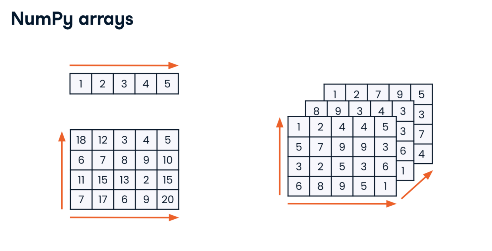
Introducing arrays

Importing NumPy
import numpy as np
Creating 1D arrays from lists
python_list = [3, 2, 5, 8, 4, 9, 7, 6, 1]
array = np.array(python_list)
array
array([3, 2, 5, 8, 4, 9, 7, 6, 1])
type(array)
numpy.ndarray
Creating 2D arrays from lists
python_list_of_lists = [[3, 2, 5],
                        [9, 7, 1],
                        [4, 3, 6]]

np.array(python_list_of_lists)
array([ [3, 2, 5],
        [9, 7, 1],
        [4, 3, 6]])
Python lists vs Numpy arrays
Python lists:- Can contain many different data types
python
  python_list = ["beep", False, 56, .945, [3, 2, 5]]
NumPy arrays:
- Can contain only a single data type
Use less space in memory
numpy_boolean_array = [[True, False], [True, True], [False, True]]
numpy_float_array = [1.9, 5.4, 8.8, 3.6, 3.2]
There are many NumPy functions used to create arrays from scratch, including:
- np.zeros()
- np.random.random()
- np.arange()
np.zeros((5, 3))
np.random.random((2, 4))
display(np.arange(-3, 4))
display(np.arange(4))
display(np.arange(-3, 4, 3))
from matplotlib import pyplot as plt
plt.scatter(np.arange(0, 7),
np.arange(-3, 4))
plt.show()

Your first NumPy array
Once you're comfortable with NumPy, you'll find yourself converting Python lists into NumPy arrays all the time for increased speed and access to NumPy's excellent array methods.
sudoku_list is a Python list containing a sudoku game:
[[0, 0, 4, 3, 0, 0, 2, 0, 9],
 [0, 0, 5, 0, 0, 9, 0, 0, 1],
 [0, 7, 0, 0, 6, 0, 0, 4, 3],
 [0, 0, 6, 0, 0, 2, 0, 8, 7],
 [1, 9, 0, 0, 0, 7, 4, 0, 0],
 [0, 5, 0, 0, 8, 3, 0, 0, 0],
 [6, 0, 0, 0, 0, 0, 1, 0, 5],
 [0, 0, 3, 5, 0, 8, 6, 9, 0],
 [0, 4, 2, 9, 1, 0, 3, 0, 0]]
You're going to change sudoku_list into a NumPy array so you can practice with it in later lessons, for example by creating a 4D array of sudoku games along with their solutions!
Instructions:
- Import NumPy using its generally accepted alias.
- Convert sudoku_list into a NumPy array called sudoku_array.
- Print the class type() of sudoku_array to check that your code has worked properly.
sudoku_list = np.array([[0, 0, 4, 3, 0, 0, 2, 0, 9],
                        [0, 0, 5, 0, 0, 9, 0, 0, 1],
                        [0, 7, 0, 0, 6, 0, 0, 4, 3],
                        [0, 0, 6, 0, 0, 2, 0, 8, 7],
                        [1, 9, 0, 0, 0, 7, 4, 0, 0],
                        [0, 5, 0, 0, 8, 3, 0, 0, 0],
                        [6, 0, 0, 0, 0, 0, 1, 0, 5],
                        [0, 0, 3, 5, 0, 8, 6, 9, 0],
                        [0, 4, 2, 9, 1, 0, 3, 0, 0]])
import numpy as np

# Convert sudoku_list into an array
sudoku_array = np.array(sudoku_list)

# Print the type of sudoku_array
print(type(sudoku_array))
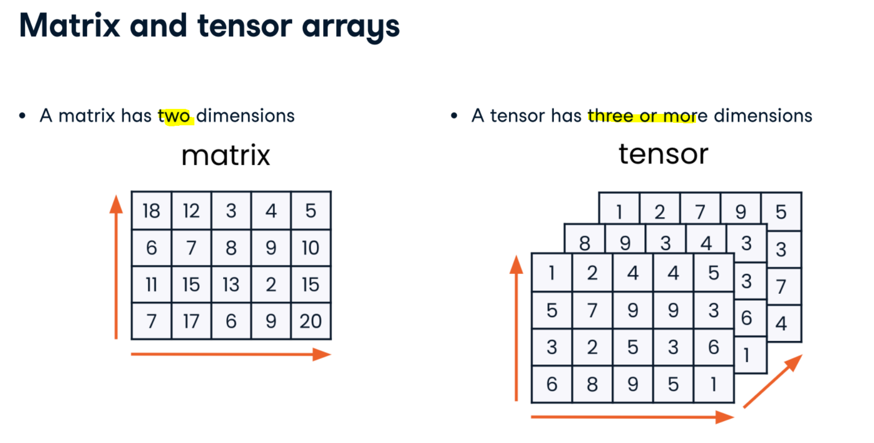
Notice that the class of sudoku_array is numpy.ndarray. ndarray is short for N-dimensional array, so-called because a NumPy array can have any number of dimensions.
Creating arrays from scratch
It can be helpful to know how to create quick NumPy arrays from scratch in order to test your code. For example, when you are doing math with large multi-dimensional arrays, it's nice to check whether the math works as expected on small test arrays before applying your code to the larger arrays. NumPy has many options for creating smaller synthetic arrays.
With this in mind, it's time for you to create some arrays from scratch! numpy is imported for you as np.
Instructions :
- Create and print an array filled with zeros called zero_array, which has two rows and four columns.
- Create and print an array of random floats between 0 and 1 called random_array, which has three rows and six columns.
zero_array = np.zeros((2, 4))
print(zero_array)

# Create an array of random floats which has six columns and three rows
random_array = np.random.random((3, 6))
print(random_array)
A range array
np.arange() has especially useful applications in graphing. Your task is to create a scatter plot with the values from doubling_array on the y-axis.
doubling_array = [1, 2, 4, 8, 16, 32, 64, 128, 256, 512]Recall that a scatter plot can be created using the following code:
plt.scatter(x_values, y_values)
plt.show()
With doubling_array on the y-axis, you now need values for the x-axis, which you can create with np.arange()!
numpy is loaded for you as np, and matplotlib.pyplot is imported as plt.
Instructions:
- Using np.arange(), create a 1D array called one_to_ten which holds all integers from one to ten (inclusive).
- Create a scatterplot with doubling_array as the y values and one_to_ten as the x values.
doubling_array = [1, 2, 4, 8, 16, 32, 64, 128, 256, 512]
one_to_ten = np.arange(1, 11)

# Create your scatterplot
plt.scatter(one_to_ten,doubling_array)
plt.show()

now you know how to make quite a range of arrays! You've also discovered that Pyplot accepts arrays as inputs, which makes sense since Matplotlib is built on top of NumPy.
array = np.zeros((3, 5))
print(array)

array.shape
array = np.array([[1, 2],
                  [5, 7],
                  [6, 6]])
array.flatten()
array = np.array([[1, 2], [5, 7], [6, 6]])
array.reshape((2, 3))
array.reshape((3, 3))
# ValueError: cannot reshape array of size 6 into shape (3,3)
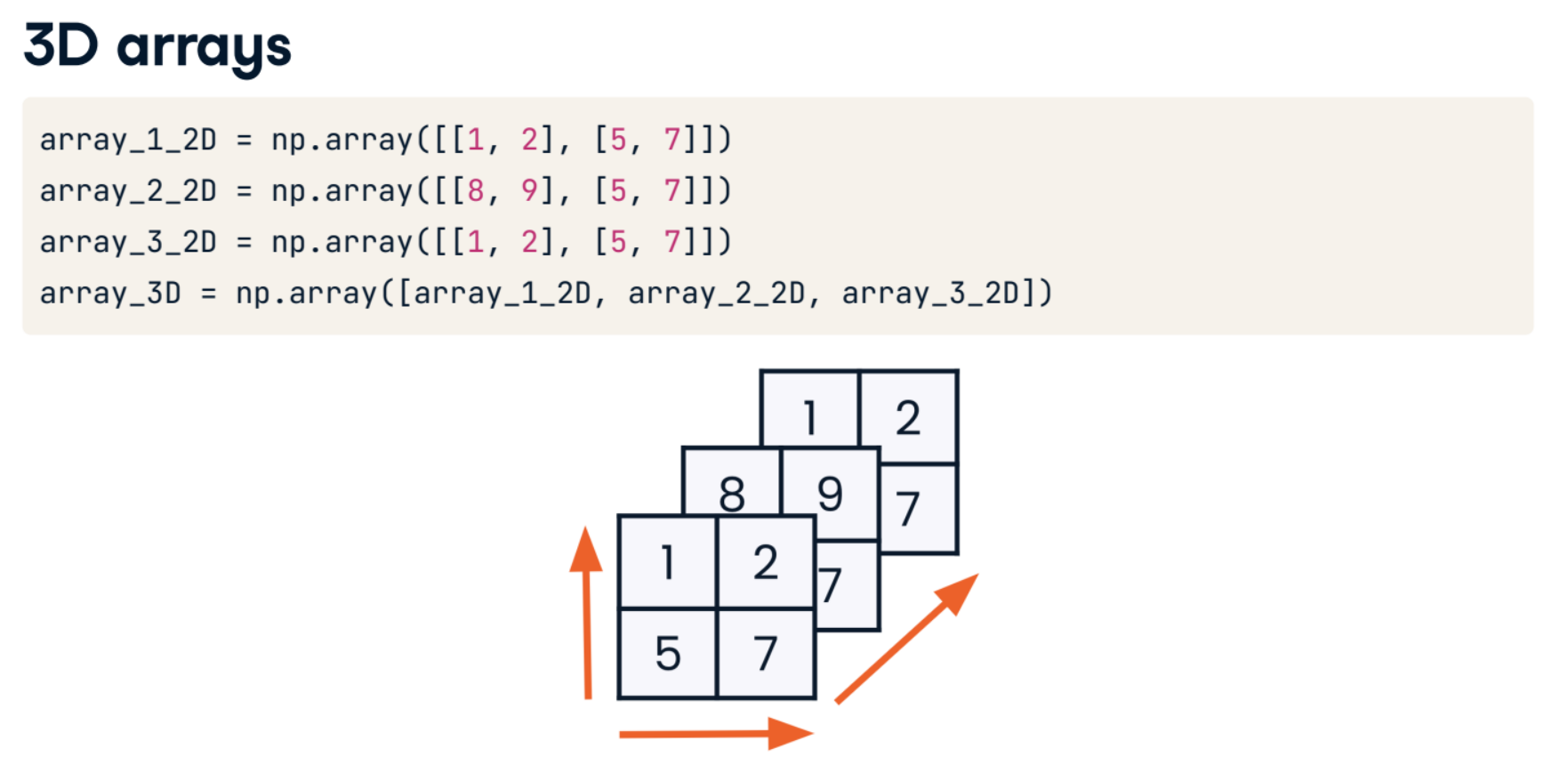
3D array creation
In the first lesson, you created a sudoku_game two-dimensional NumPy array. Perhaps you have hundreds of sudoku game arrays, and you'd like to save the solution for this one, sudoku_solution, as part of the same array as its corresponding game in order to organize your sudoku data better. You could accomplish this by stacking the two 2D arrays on top of each other to create a 3D array.
numpy is loaded as np, and the sudoku_game and sudoku_solution arrays are available.
Instructions:
- Create a 3D array called game_and_solution by stacking the two 2D arrays, sudoku_game and sudoku_solution, on top of one another; in the final array, sudoku_game should appear before sudoku_solution.
- Print game_and_solution.
game_and_solution = np.array([sudoku_game,sudoku_solution ])

# Print game_and_solution
print(game_and_solution)
Notice how storing sudoku_game and sudoku_solution in three dimensions makes more sense than adding the data from both to one 2D array.
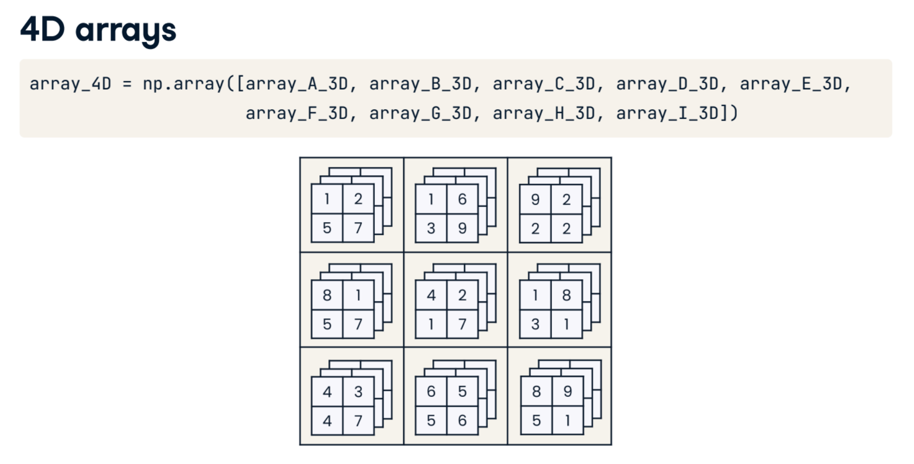
The fourth dimension
Printing arrays is a good way to check code output for small arrays like sudoku_game_and_solution, but it becomes unwieldy when dealing with bigger arrays and those with higher dimensions. Another important check is to look at the array's .shape.
Now, you'll create a 4D array that contains two sudoku games and their solutions. numpy is loaded as np. The game_and_solution 3D array you created in the previous example is available, along with new_sudoku_game and new_sudoku_solution.
Instructions:
- Create another 3D array called new_game_and_solution with a different 2D game and 2D solution pair: new_sudoku_game and new_sudoku_solution. new_sudoku_game should appear before new_sudoku_solution.
- Create a 4D array called games_and_solutions by making an array out of the two 3D arrays: game_and_solution and new_game_and_solution, in that order.
- Print the shape of games_and_solutions.
game_and_solution = np.array([  [[0, 0, 4, 3, 0, 0, 2, 0, 9],
                                [0, 0, 5, 0, 0, 9, 0, 0, 1],
                                [0, 7, 0, 0, 6, 0, 0, 4, 3],
                                [0, 0, 6, 0, 0, 2, 0, 8, 7],
                                [1, 9, 0, 0, 0, 7, 4, 0, 0],
                                [0, 5, 0, 0, 8, 3, 0, 0, 0],
                                [6, 0, 0, 0, 0, 0, 1, 0, 5],
                                [0, 0, 3, 5, 0, 8, 6, 9, 0],
                                [0, 4, 2, 9, 1, 0, 3, 0, 0]],

                                [[8, 6, 4, 3, 7, 1, 2, 5, 9],
                                [3, 2, 5, 8, 4, 9, 7, 6, 1],
                                [9, 7, 1, 2, 6, 5, 8, 4, 3],
                                [4, 3, 6, 1, 9, 2, 5, 8, 7],
                                [1, 9, 8, 6, 5, 7, 4, 3, 2],
                                [2, 5, 7, 4, 8, 3, 9, 1, 6],
                                [6, 8, 9, 7, 3, 4, 1, 2, 5],
                                [7, 1, 3, 5, 2, 8, 6, 9, 4],
                                [5, 4, 2, 9, 1, 6, 3, 7, 8]]])
new_sudoku_game = np.array([[0, 0, 4, 3, 0, 0, 0, 0, 0],
                            [8, 9, 0, 2, 0, 0, 6, 7, 0],
                            [7, 0, 0, 9, 0, 0, 0, 5, 0],
                            [5, 0, 0, 0, 0, 8, 1, 4, 0],
                            [0, 7, 0, 0, 3, 2, 0, 6, 0],
                            [6, 0, 0, 0, 0, 1, 3, 0, 8],
                            [0, 0, 1, 7, 5, 0, 9, 0, 0],
                            [0, 0, 5, 0, 4, 0, 0, 1, 2],
                            [9, 8, 0, 0, 0, 6, 0, 0, 5]])

new_sudoku_solution = np.array([[2, 5, 4, 3, 6, 7, 8, 9, 1],
                                [8, 9, 3, 2, 1, 5, 6, 7, 4],
                                [7, 1, 6, 9, 8, 4, 2, 5, 3],
                                [5, 3, 2, 6, 9, 8, 1, 4, 7],
                                [1, 7, 8, 4, 3, 2, 5, 6, 9],
                                [6, 4, 9, 5, 7, 1, 3, 2, 8],
                                [4, 2, 1, 7, 5, 3, 9, 8, 6],
                                [3, 6, 5, 8, 4, 9, 7, 1, 2],
                                [9, 8, 7, 1, 2, 6, 4, 3, 5]])
new_game_and_solution = np.array([new_sudoku_game , new_sudoku_solution])

# Create a 4D array of both game and solution 3D arrays
games_and_solutions = np.array([game_and_solution , new_game_and_solution])

# Print the shape of your 4D array
print(games_and_solutions.shape)
Fabulous 4D array! The .shape of (2, 2, 9, 9) means that there are two sets of game/solution pairs. Within each game/solution pair, all arrays have nine rows and nine columns. That's exactly right! If there were ten game/solution pairs, the .shape would be (10, 2, 9, 9).
Flattening and reshaping
You've learned to change not only array shape but also the number of dimensions that an array has. To test these skills, you'll change sudoku_game from a 2D array to a 1D array and back again. Can we trust NumPy to keep the array elements in the same order after being flattened and reshaped? Time to find out.
numpy is imported as np, and sudoku_game is loaded for you.
Instructions:
- Flatten sudoku_game so that it is a 1D array, and save it as flattened_game.
- Print the .shape of flattened_game.
- Reshape the flattened_game back to its original shape of nine rows and nine columns; save the new array as reshaped_game.
flattened_game = sudoku_game.flatten()

# Print the shape of flattened_game
print(flattened_game.shape)

# Reshape flattened_game back to a nine by nine array
reshaped_game = flattened_game.reshape(9,9)

# Print sudoku_game and reshaped_game
print(sudoku_game)
print(reshaped_game)
Nice work resurrecting that sudoku game. Notice that .flatten() preserves the order of array elements—when the array is reshaped back to its original shape, the numbers are in the exact same places as they were before flattening.
np.array([1.32, 5.78, 175.55]).dtype
int_array = np.array([[1, 2, 3], [4, 5, 6]])
int_array.dtype
np.array(["Introduction", "to", "NumPy"]).dtype
float32_array = np.array([1.32, 5.78, 175.55], dtype=np.float32)
float32_array.dtype
boolean_array = np.array([[True, False], [False, False]], dtype=np.bool_)
array = boolean_array.astype(np.int32)
array.dtype
np.array([True, "Boop", 42, 42.42]) # all become string type (biggest size)
# Adding a .oat to an array of integers will change all integers into .oats:
np.array([0, 42, 42.42]).dtype
# Adding an integer to an array of booleans will change all booleans in to integers:
np.array([True, False, 42]).dtype
The dtype argument
One way to control the data type of a NumPy array is to declare it when the array is created using the dtype keyword argument. Take a look at the data type NumPy uses by default when creating an array with np.zeros(). Could it be updated?
numpy is loaded as np.
Instructions:
- Using np.zeros(), create an array of zeros that has three rows and two columns; call it zero_array.
- Print the data type of zero_array.
- Create a new array of zeros called zero_int_array, which will also have three rows and two columns, but the data type should be np.int32.
- Print the data type of zero_int_array.
zero_array = np.zeros((3, 2))

# Print the data type of zero_array
print(zero_array.dtype)

# Create a new array of int32 zeros with three rows and two columns
zero_int_array = np.zeros((3,2), dtype = np.int32)

# Print the data type of zero_int_array
print(zero_int_array.dtype)
Since your original zero_array did not have any information following the decimal places of the floats, it makes sense to change the array's data type to an integer with a smaller bitsize.
A smaller sudoku game
NumPy data types, which emphasize speed, are more specific than Python data types, which emphasize flexibility. When working with large amounts of data in NumPy, it's good practice to check the data type and consider whether a smaller data type is large enough for your data, since smaller data types use less memory.
It's time to make your sudoku game more memory-efficient using your knowledge of data types! sudoku_game has been loaded for you as a NumPy array. numpy is imported as np
- Change the data type of sudoku_game to be int8, an 8-bit integer; name the new array small_sudoku_game.
- Print the data type of small_sudoku_game to be sure that your change to int8 is reflected.
print(sudoku_game.dtype)

# Change the data type of sudoku_game to int8
small_sudoku_game = sudoku_game.astype(np.int8)

# Print the data type of small_sudoku_game
print(small_sudoku_game.dtype)
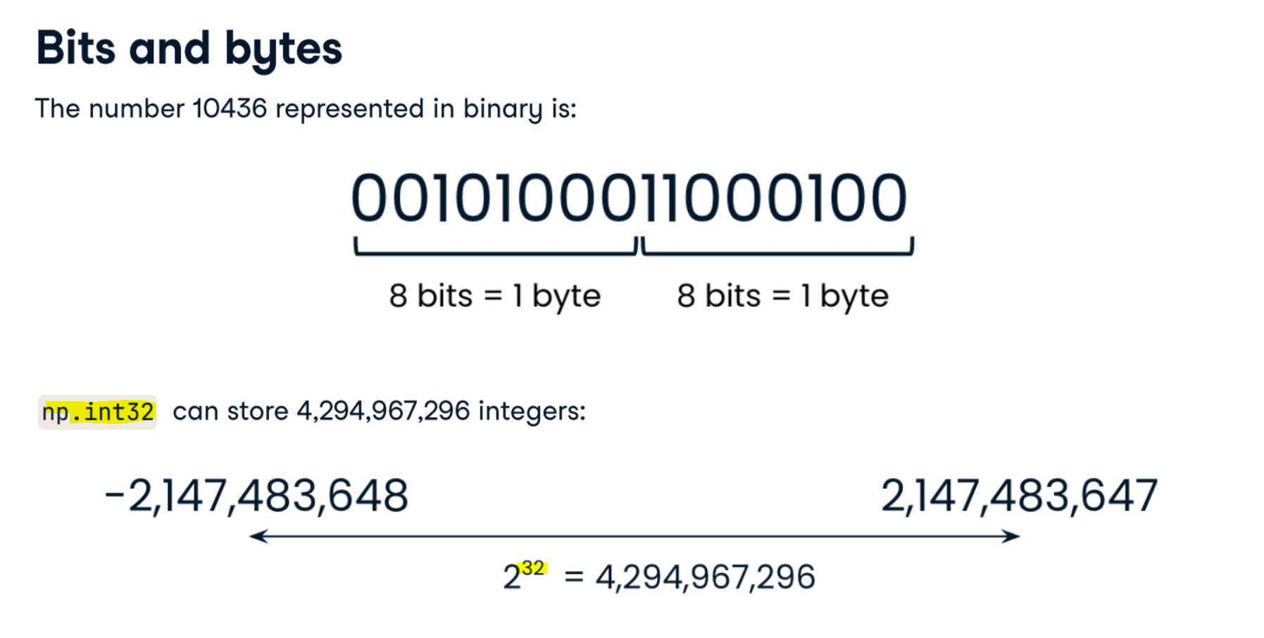
Gr8 data type casting! int8 is one of the smallest data types in NumPy since 8 bits is only a single byte.
Selecting and Updating Data
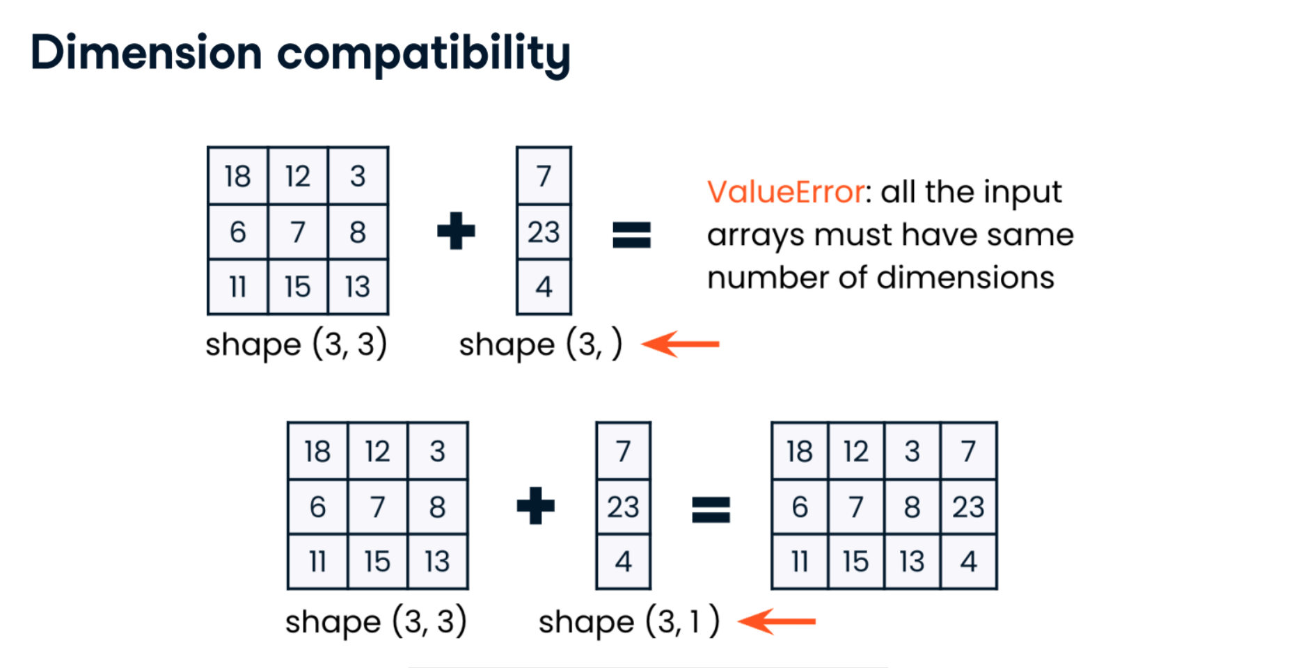
Sharpen your NumPy data wrangling skills by slicing, filtering, and sorting New York City’s tree census data. Create new arrays by pulling data based on conditional statements, and add and remove data along any dimension to suit your purpose. Along the way, you’ll learn the shape and dimension compatibility principles to prepare for super-fast array math.
array = np.array([2, 4, 6, 8, 10])
array[3]
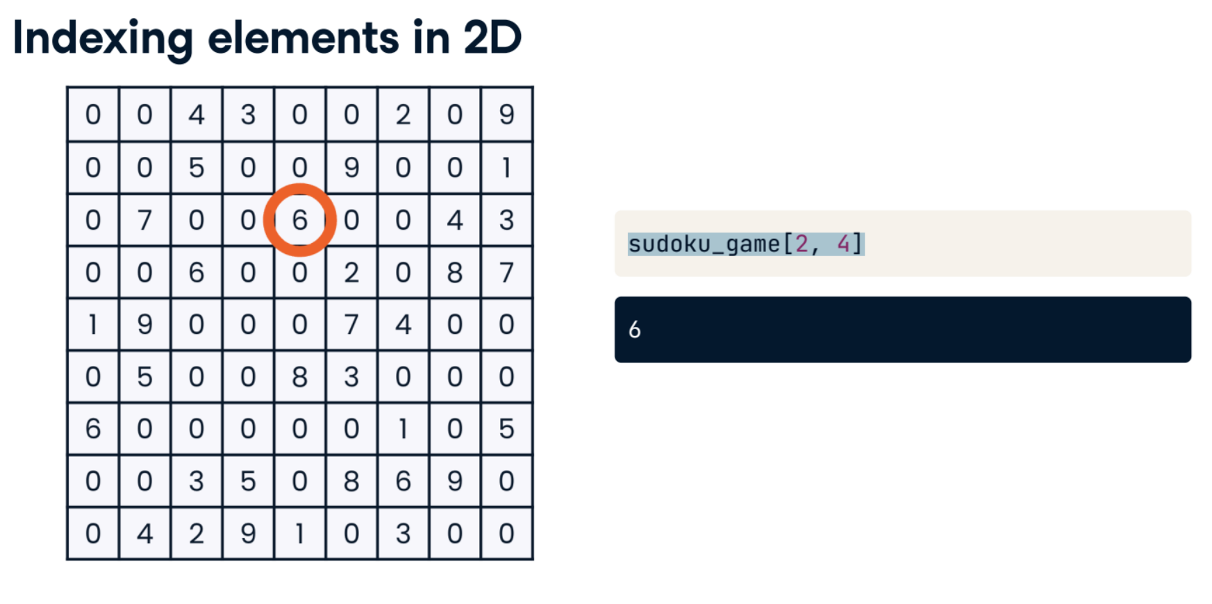
sudoku_game[2, 4]
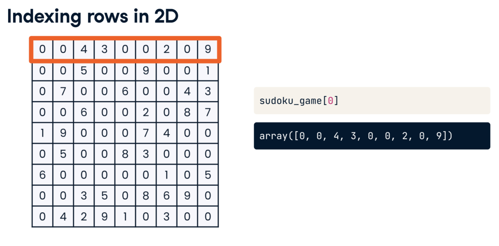
sudoku_game[0]
array = np.array([2, 4, 6, 8, 10])
array[2:4]
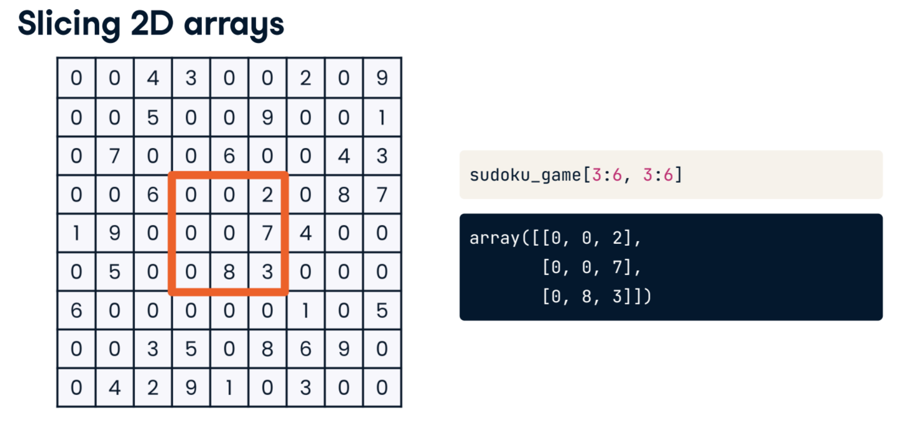
sudoku_game[3:6, 3:6]
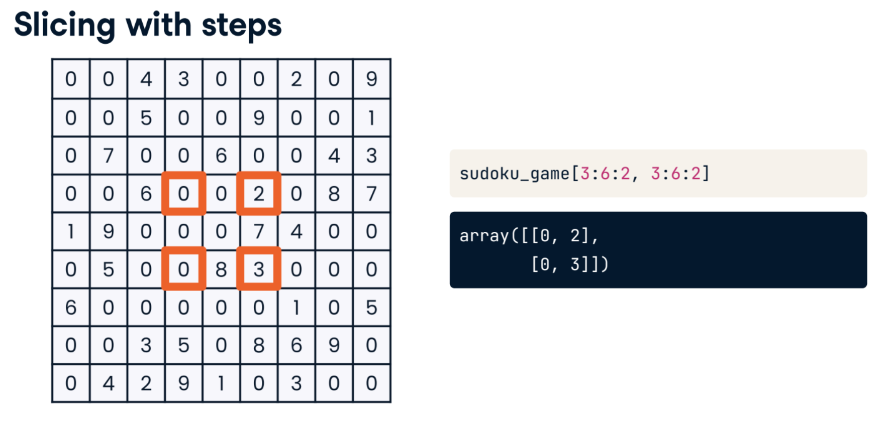
sudoku_game[3:6:2, 3:6:2]
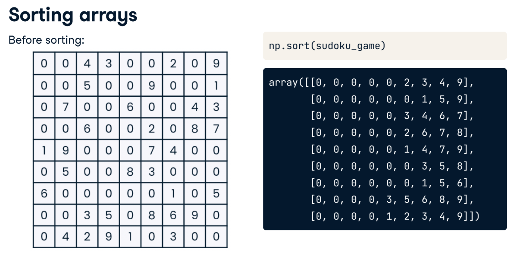
np.sort(sudoku_game)
sudoku_game
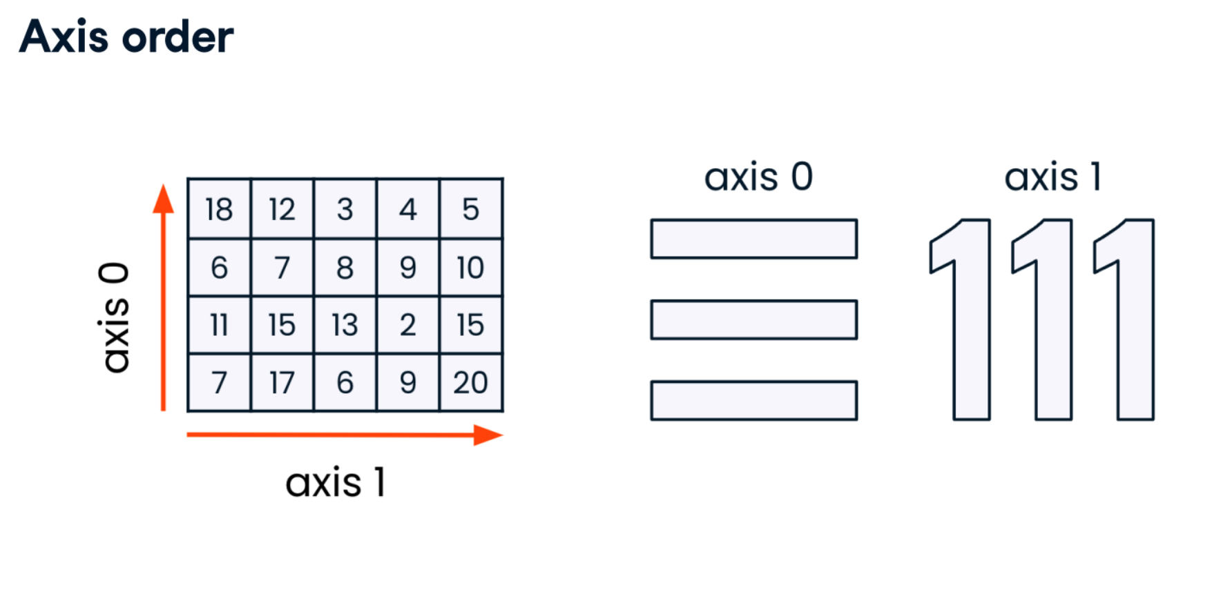
np.sort(sudoku_game, axis=0)
Slicing and indexing trees
Imagine you are a researcher working with data from New York City's tree census. Each row of the tree_census 2D array lists information for a different tree: the tree ID, block ID, trunk diameter, and stump diameter in that order. Living trees do not have stump diameters, which explains why there are so many zeros in that column. Column order is important because NumPy does not have column names! The first and last three rows of tree_census are shown below.
array([[     3, 501451,     24,      0],
       [     4, 501451,     20,      0],
       [     7, 501911,      3,      0],
       ...,
       [  1198, 227387,     11,      0],
       [  1199, 227387,     11,      0],
       [  1210, 227386,      6,      0]])
In this exercise, you'll be working specifically with the second column, representing block IDs: your research requires you to select specific city blocks for further analysis using NumPy slicing and indexing. numpy is loaded as np, and the tree_census 2D array is available.
Instructions:
- Select all rows of data from the second column, representing block IDs; save the resulting array as block_ids.
- Print the first five block IDs from block_ids.
- Select the tenth block ID from block_ids, saving the result as tenth_block_id.
- Select five consecutive block IDs from block_ids, starting with the tenth ID, and save as block_id_slice
block_ids = tree_census[:,1]

# Print the first five block_ids
print(block_ids[:5])
block_ids = tree_census[:, 1]

# Select the tenth block ID from block_ids
tenth_block_id = block_ids[9]
print(tenth_block_id)
block_ids = tree_census[:, 1]

# Select five block IDs from block_ids starting with the tenth ID
block_id_slice = block_ids[9:9+5]
print(block_id_slice)
No mental block for you! Well done. Notice how the slicing and indexing syntax for a 1D array is exactly as it would be if you were working with a Python list!
Stepping into 2D
Now assume that your research requires you to take an admittedly unrepresentative sample of trunk diameters, which are located in the third column of tree_census. Getting just a selection of trunk diameters can be done with NumPy's slicing and stepping functionality.
numpy is loaded as np, and the tree_census 2D array is available.
Instructions:
- Create an array called hundred_diameters which contains the first 100 trunk diameters in tree_census.
- Create an array,every_other_diameter, which contains only every other trunk diameter for trees with row indices from 50 to 100, inclusive.
hundred_diameters = tree_census[:100,2]
print(hundred_diameters)
every_other_diameter = tree_census[50:101:2, 2]
print(every_other_diameter)
Look at that slicing! Great work. Notice how you only sliced the rows. In terms of columns, you just indicated that you were working with the column at index two: trunk diameter.
Sorting trees
Sometimes it's easiest to understand data when it is sorted according to the value you are most interested in. Your new research task is to create an array containing the trunk diameters in the New York City tree census, sorted in order from smallest to largest.
numpy is loaded as np, and the tree_census 2D array is available.
Instructions:
- Create an array called sorted_trunk_diameters which selects only the trunk diameter column from tree_census and sorts it so that the smallest trunk diameters are at the top of the array and the largest at the bottom.
sorted_trunk_diameters = np.sort(tree_census[:, 2])
print(sorted_trunk_diameters)
Way to get to the root of that tree problem! Notice that the np.sort()function doesn't include an option to sort ascending or descending.
Filtering arrays
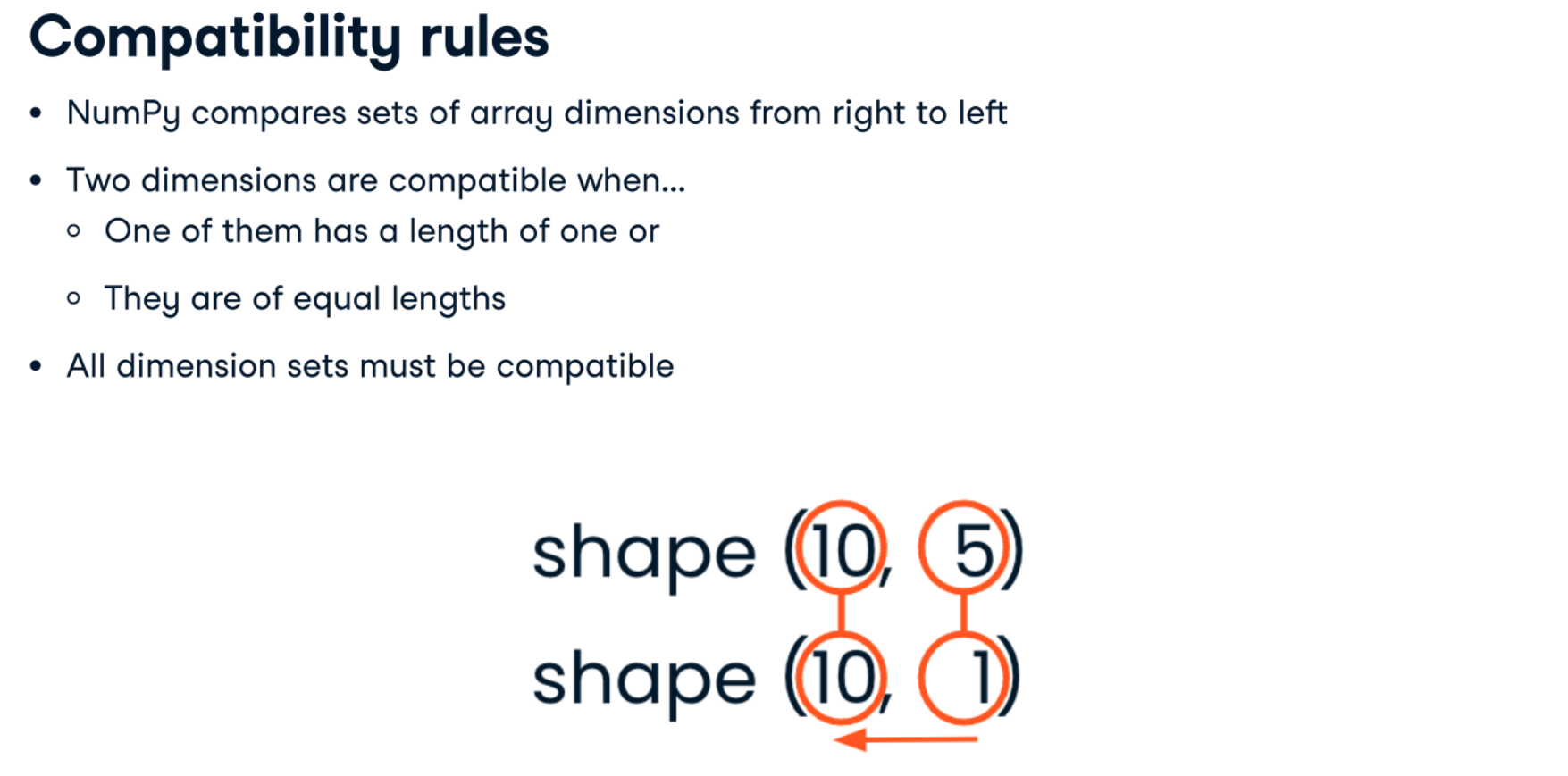
Two ways to filter
- Masks and fancy indexing
- np.where()
Boolean masks
one_to_five = np.arange(1, 6)
one_to_five
# array([1, 2, 3, 4, 5])

mask = one_to_five % 2 == 0
mask
# array([False, True, False, True, False])
- Filtering with fancy indexing
one_to_five = np.arange(1, 6)
mask = one_to_five % 2 == 0

one_to_five[mask]
# array([2, 4])
- 2D fancy indexing
classroom_ids_and_sizes = np.array([[1, 22], [2, 21], [3, 27], [4, 26]])
classroom_ids_and_sizes
classroom_ids_and_sizes[:, 1] % 2 == 0
classroom_ids_and_sizes[:, 0][classroom_ids_and_sizes[:, 1] % 2 == 0]
Fancy indexing vs. np.where()
Fancy indexing
- Returns array of elements
- Returns array of elements
np.where()
- Returns array of indices
- Can create an array based on whether
- elements do or don't meet condition
- Filtering with np.where()
classroom_ids_and_sizes
np.where(classroom_ids_and_sizes[:, 1] % 2 == 0) # np.where return a tuple of array
sudoku_game
row_ind, column_ind = np.where(sudoku_game == 0)
row_ind, column_ind
np.where(sudoku_game == 0, "", sudoku_game)
Filtering with masks
In the last lesson, you sorted trees from smallest to largest. Now, you'll use fancy indexing to return the row of data representing the largest tree in tree_census. You'll also examine other trees located on the same block as the largest tree: are they also large?
numpy is loaded as np, and the tree_census array is available. As a reminder, the tree_census columns in order refer to a tree's ID, its block ID, its trunk diameter, and its stump diameter.
Instructions:
- Using Boolean indexing, create an array, largest_tree_data, which contains the row of data on the largest tree in tree_census corresponding to the tree with a diameter of 51.
- Slice largest_tree_data to retrieve only the block id of the block the largest tree is located on; save this block id as largest_tree_block_id.
- Using fancy indexing, create an array called trees_on_largest_tree_block which contains data on all trees with the same block ID as the largest tree.
largest_tree_data = tree_census[tree_census[:, 2] == 51]
print(largest_tree_data)

# Slice largest_tree_data to get only the block ID
largest_tree_block_id = largest_tree_data[:, 1]
print(largest_tree_block_id)

# Create an array which contains row data on all trees with largest_tree_block_id
trees_on_largest_tree_block = tree_census[tree_census[:, 1] == largest_tree_block_id]
print(trees_on_largest_tree_block)
Based on your work, it looks like the largest tree on the tree_census is the only really big tree on its block.
Fancy indexing vs. np.where()
ou and your tree research team are double-checking collection data by visiting a few trees in person to confirm their measurements. You've been assigned to check the data for trees on block 313879, and you'd like to make a small array of just the tree data that relates to your work.
numpy is loaded as np, and the tree_census array is available. As a reminder, the tree_census columns in order refer to a tree's ID, its block ID, its trunk diameter, and its stump diameter.
Instructions:
- Using fancy indexing, create an array called block_313879 which only contains data for trees with a block ID of 313879.
block_313879 = tree_census[tree_census[:, 1] ==  313879]
print(block_313879)
- Using np.where(), create an array of row_indices for trees with a block ID of 313879.
- Using row_indices, create block_313879, which contains data for trees on block 313879.
row_indices = np.where(tree_census[:,1] == 313879)

# Create an array which only contains data for trees on block 313879
block_313879 = tree_census[row_indices]
print(block_313879)
Great filtering. You probably noticed that fancy indexing is more elegant than np.where() in this example. That's because we haven't really tapped into the power of np.where() yet. It's most useful for finding indices and then using that location information to update an array. We'll see an example of this in the next exercise, and also in the next lesson, where one of the functions takes indices as arguments!
Creating arrays from conditions
Currently, the stump diameter and trunk diameter values in tree_census are in two different columns. Living trees have a stump diameter of zero while stumps have a trunk diameter of zero. If you'd like to include both living trees and stumps in certain research calculations, it might be useful to have their diameters together in just one column.
numpy is loaded as np, and the tree_census array is available. As a reminder, the tree census columns in order refer to a tree's ID, its block ID, its trunk diameter, and its stump diameter.
Instructions:
- Create and print a 1D array called trunk_stump_diameters, which replaces a tree's trunk diameter with its stump diameter if the trunk diameter is zero.
trunk_stump_diameters = np.where(tree_census[:,2] == 0,tree_census[:,3], tree_census[:,2] )
print(trunk_stump_diameters)
But this is just a 1D array without any tree or block ID information. How do we add this information back to the tree_census array? That's the subject of our next lesson!
classroom_ids_and_sizes = np.array([[1, 22], [2, 21], [3, 27], [4, 26]])
new_classrooms = np.array([[5, 30], [5, 17]])
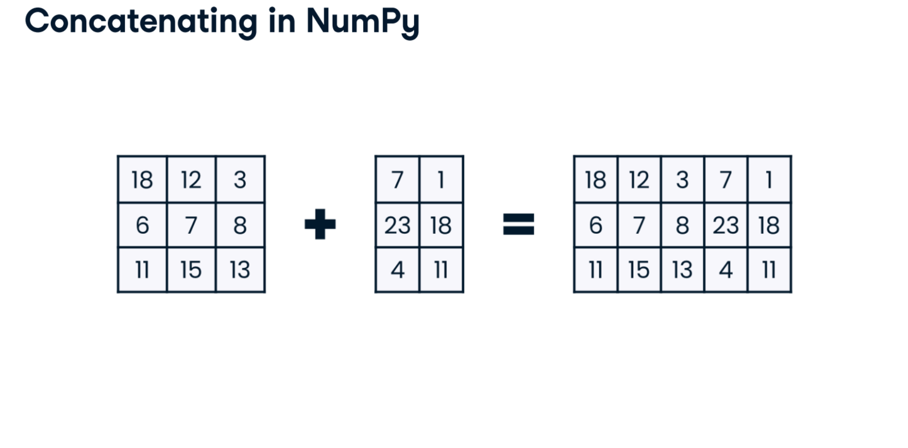
np.concatenate((classroom_ids_and_sizes, new_classrooms))
- Concatenating columns
- Specify the
axis = 1
- Specify the
classroom_ids_and_sizes = np.array([[1, 22], [2, 21], [3, 27], [4, 26]])
grade_levels_and_teachers = np.array([[1, "James"], [1, "George"], [3,"Amy"],[3, "Meehir"]])
classroom_data = np.concatenate((classroom_ids_and_sizes, grade_levels_and_teachers), axis=1)
classroom_data
array_1D = np.array([1, 2, 3])
column_array_2D = array_1D.reshape((3, 1))
display(column_array_2D)

row_array_2D = array_1D.reshape((1, 3))
display(row_array_2D)

classroom_data
- Deleting with np.delete()
np.delete(classroom_data, 1, axis=0)
- Deleting columns
np.delete(classroom_data, 1, axis=1)
- Deleting without an axis
- Numpy will delete at the index of the flatten version of the array.
classroom_data
np.delete(classroom_data, 1)
Adding rows
The research team has discovered two trees that were left off the tree_census. Your task is to add rows containing the data for these new trees to the end of the tree_census array. The new trees' data is saved in a 2D array called new_trees:
numpy is loaded as np, and the tree_census and new_trees arrays are available.
Instructions:
- Add rows to the end of tree_census containing data for the new trees from the new_trees 2D array; save the new array as updated_tree_census.
new_trees = np.array([[1211, 227386, 20, 0], [1212, 227386, 8, 0]])
print(tree_census.shape, new_trees.shape)

# Add rows to tree_census which contain data for the new trees
updated_tree_census = np.concatenate((tree_census, new_trees))
print(updated_tree_census)
Adding columns
You finished the last set of exercises by creating an array called trunk_stump_diameters, which combined data from the trunk diameter and stump diameter columns into a 1D array. Now, you'll add that 1D array as a column to the tree_census array.
numpy is loaded as np, and both the tree_census and trunk_stump_diameters arrays are available.
Instructions:
- Print the shapes of both tree_census and trunk_stump_diameters.
- Reshape trunk_stump_diameters so that it can be appended as the last column in tree_census; call the reshaped array reshaped_diameters.
- Concatenate reshaped_diameters to the end of tree_census so that it becomes the last column; call the new array concatenated_tree_census.
print(trunk_stump_diameters.shape, tree_census.shape)

# Reshape trunk_stump_diameters
reshaped_diameters = trunk_stump_diameters.reshape((1000, 1))

# Concatenate reshaped_diameters to tree_census as the last column
concatenated_tree_census = np.concatenate((tree_census, reshaped_diameters), axis = 1)
print(concatenated_tree_census)
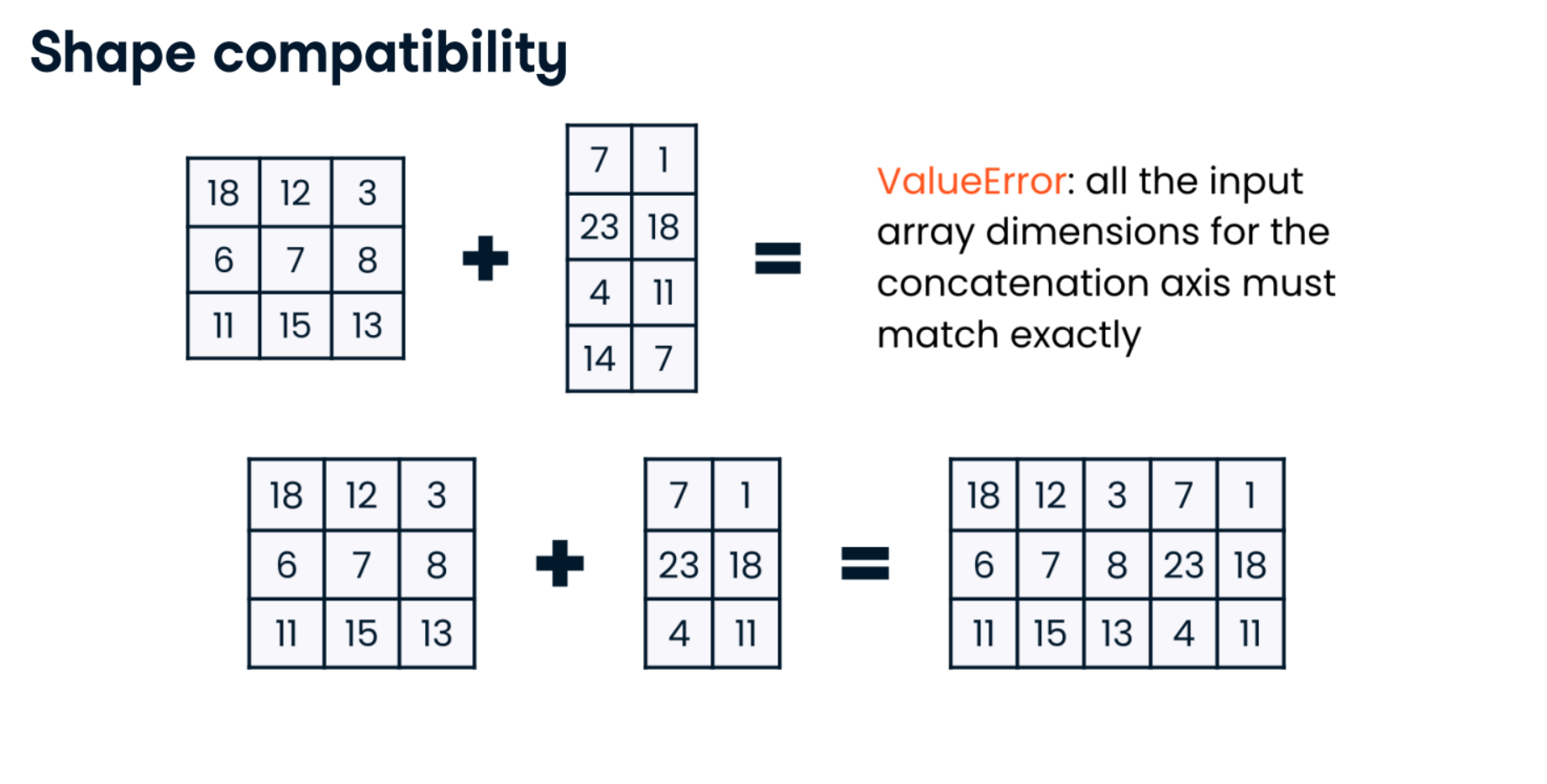
That's right! Adding a 1D array to an existing 2D array requires you to reshape the 1D array into a 2D array first. We'll dive into shape compatibility issues like this even further in the next chapter on array mathematics!
Deleting with np.delete()
What if your tree research focuses only on living trees on publicly-owned city blocks? It might be helpful to delete some unneeded data like the stump diameter column and some trees located on private blocks.
You've learned that NumPy's np.delete() function takes three arguments: the original array, the index or indices to be deleted, and the axis to delete along. If you don't know the index or indices of the array you'd like to delete, recall that when it is only passed one argument,np.where() returns an array of indices where a condition is met!
numpy is loaded as np, and the tree_census 2D array is available. The columns in order refer to a tree's ID, block number, trunk diameter, and stump diameter.
Instructions:
- Delete the stump diameter column from tree_census, and save the new 2D array as tree_census_no_stumps.
- Using np.where(), find the indices of any trees on block 313879, a private block. Save the indices in an array called private_block_indices.
- Using the indices you just found using np.where(), delete the rows for trees on block 313879 from tree_census_no_stumps, saving the new 2D array as tree_census_clean.
- Print the shape of tree_census_clean.
tree_census_no_stumps = np.delete(tree_census, 3, axis=1)

# Save the indices of the trees on block 313879
private_block_indices = np.where(tree_census[:,1] == 313879)

# Delete the rows for trees on block 313879 from tree_census_no_stumps
tree_census_clean = np.delete(tree_census_no_stumps, private_block_indices, axis=0)

# Print the shape of tree_census_clean
print(tree_census_clean.shape)
We can't stump you! Notice that the new shape reflects two fewer rows and one fewer column than tree_census started with because of your deletions: just as expected.
Array Mathematics!
Leverage NumPy’s speedy vectorized operations to gather summary insights on sales data for American liquor stores, restaurants, and department stores. Vectorize Python functions for use in your NumPy code. Finally, use broadcasting logic to perform mathematical operations between arrays of different sizes.
Summarizing data
Aggregating methods
.sum().min().max().mean().cumsum()
- Summing data
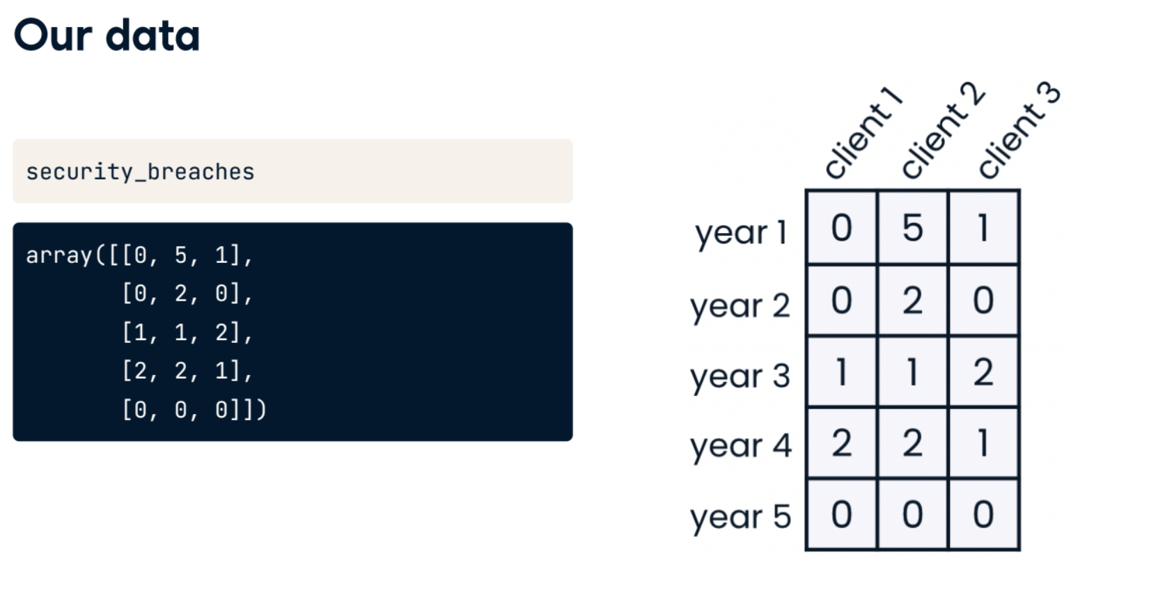
security_breaches = np.array([[0, 5, 1],
                              [0, 2, 0],
                              [1, 1, 2],
                              [2, 2, 1],
                              [0, 0, 0]])

security_breaches.sum()
- Aggregating Rows
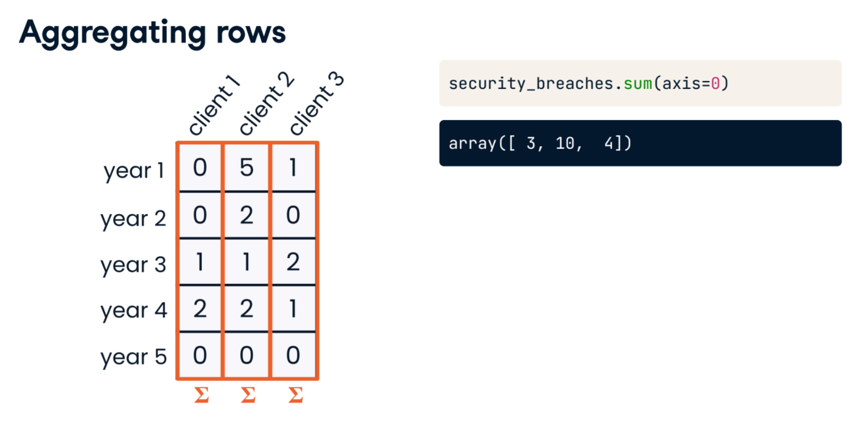
security_breaches.sum(axis=0)
- Aggregating columns
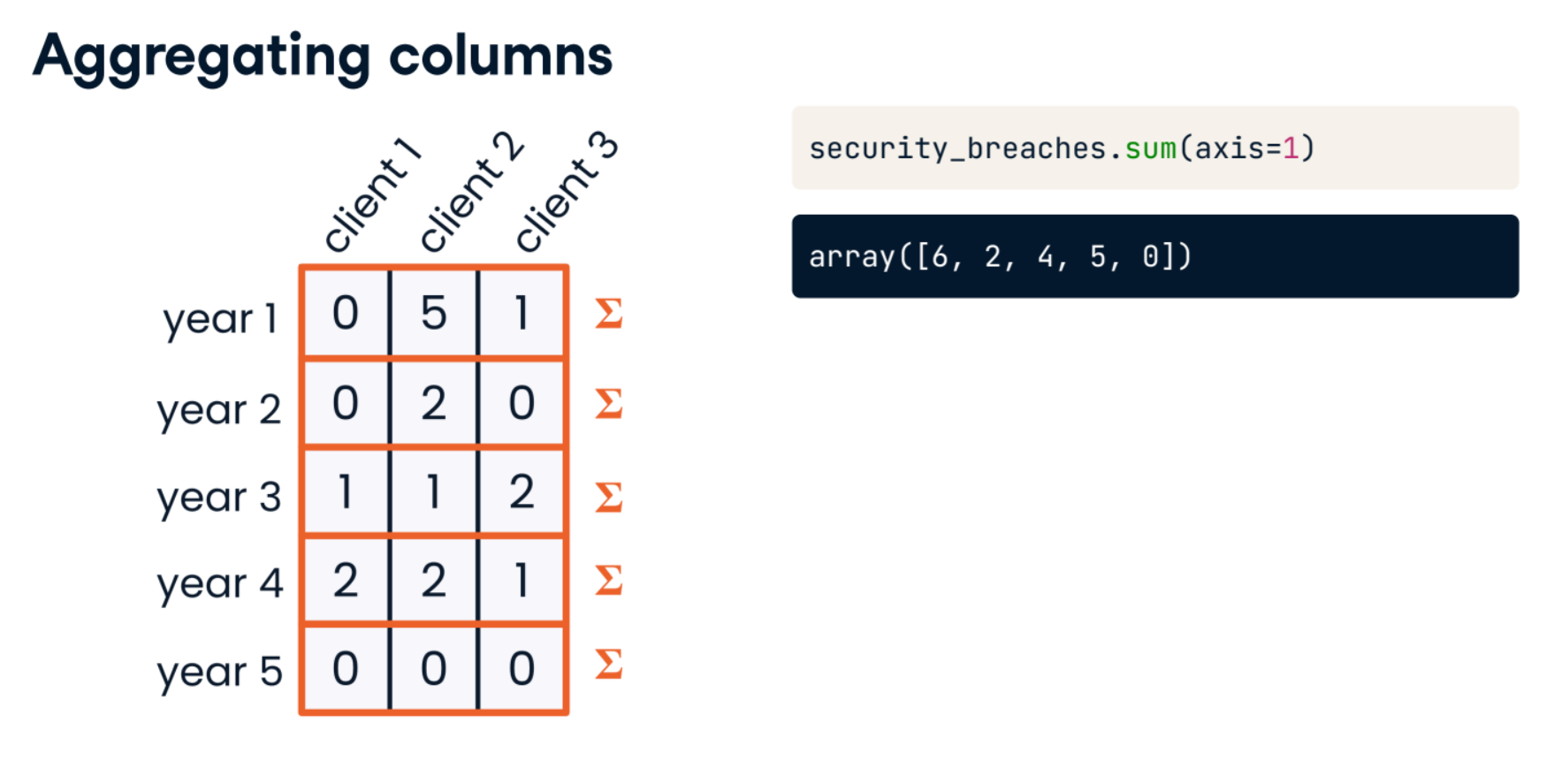
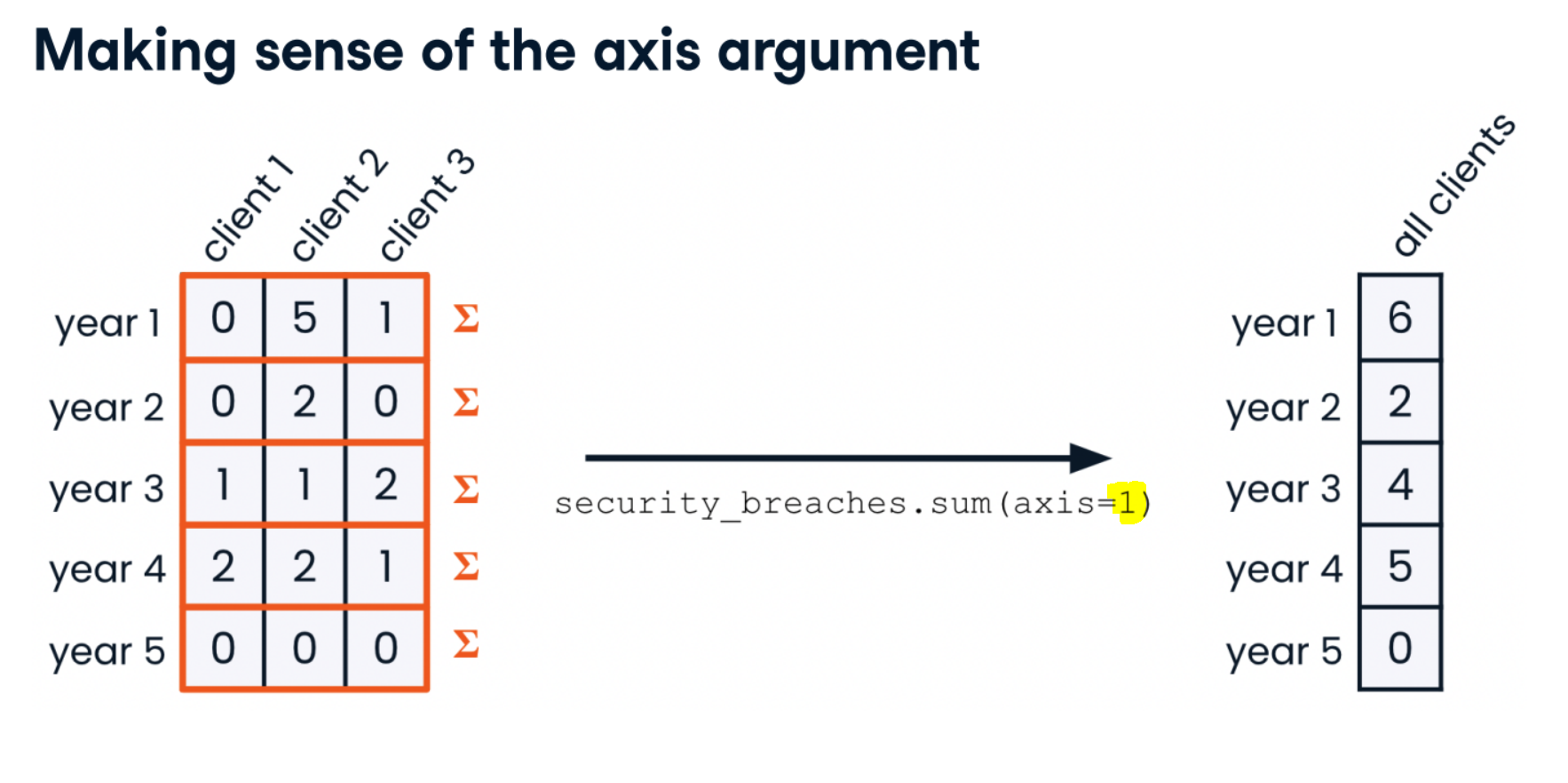
security_breaches.sum(axis=1)
- Minimum and maximum values
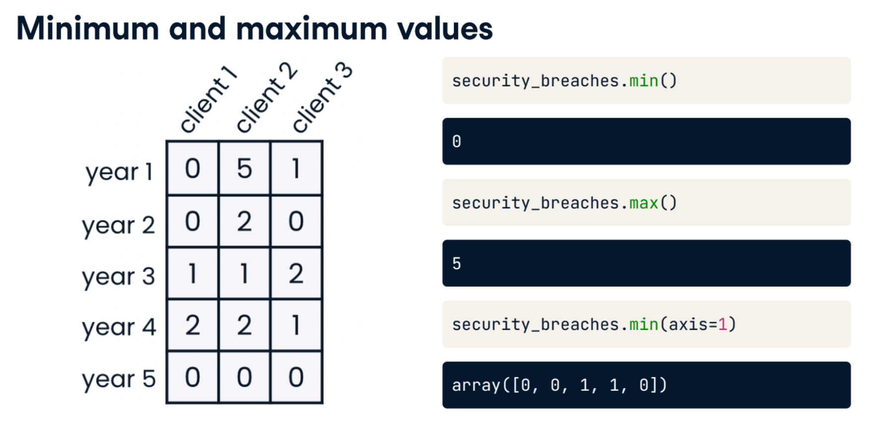
display(security_breaches.min())
display(security_breaches.max())
display(security_breaches.min(axis=1))
- Finding the mean
print(security_breaches.mean())
display(security_breaches.mean(axis=1))
- The keepdims argument
display(security_breaches.sum(axis=1))
display(security_breaches.sum(axis=1, keepdims=True)) # keep the dimension, already is the 2D array.
- Cumulative sums
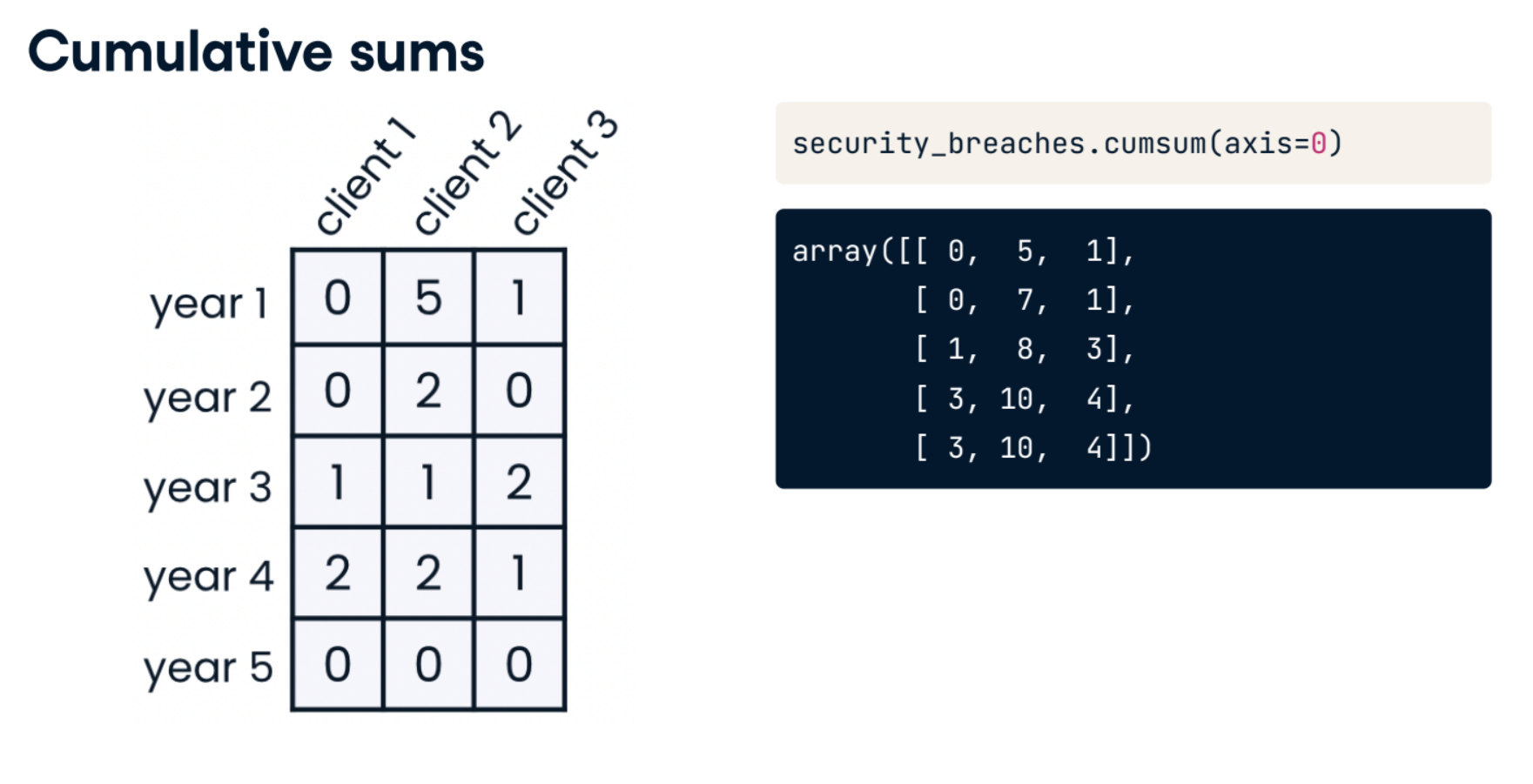
security_breaches.cumsum(axis=0)
- Graphing summary values
cum_sums_by_client = security_breaches.cumsum(axis=0)
plt.plot(np.arange(1, 6), cum_sums_by_client[:, 0], label="Client 1")
plt.plot(np.arange(1, 6), cum_sums_by_client.mean(axis=1), label="Average")
plt.legend()
plt.show()

Sales totals
The dataset you'll be working with during this chapter is one year's sales data by month for three different industries. Each row in this monthly_sales array represents a month from January to December. The first column has monthly sales data for liquor stores, the second column has data for restaurants, and the last column tracks sales for department stores.
array([[ 4134, 23925,  8657],
       [ 4116, 23875,  9142],
       [ 4673, 27197, 10645],
       [ 4580, 25637, 10456],
       [ 5109, 27995, 11299],
       [ 5011, 27419, 10625],
       [ 5245, 27305, 10630],
       [ 5270, 27760, 11550],
       [ 4680, 24988,  9762],
       [ 4913, 25802, 10456],
       [ 5312, 25405, 13401],
       [ 6630, 27797, 18403]])
Your task is to create an array with all the information from monthly_sales as well as a fourth column which totals the monthly sales across industries for each month.
numpy is loaded for you as np, and the monthly_sales array is available.
Instructions:
- Create a 2D array which contains a single column of total monthly sales across industries; call it monthly_industry_sales.
- Concatenate monthly_industry_sales with monthly_sales into a new array called monthly_sales_with_total, with the monthly cross-industry sales information in the final column.
monthly_industry_sales = monthly_sales.sum(axis=1, keepdims=True)
print(monthly_industry_sales)

# Add this column as the last column in monthly_sales
monthly_sales_with_total = np.concatenate((monthly_sales, monthly_industry_sales), axis = 1)
print(monthly_sales_with_total)
Those are sum good-looking arrays! Notice how using the keepdims keyword is helpful not only for dimension compatibility but also for visualizing which axis your aggregating data originates from!
Plotting averages
Perhaps you have a hunch that department stores see greater increased sales than average during the end of the year as people rush to buy gifts. You'd like to test this theory by comparing monthly department store sales to average sales across all three industries.
numpy is loaded for you as np, and the monthly_sales array is available. The monthly_sales columns in order refer to liquor store, restaurant, and department store sales.
Instructions:
- Plot an array of the numbers one through twelve (representing each month) on the x-axis and avg_monthly_sales on the y-axis.
- Plot an array of the numbers one through twelve on the x-axis and the department store sales column of monthly_sales on the y-axis.
avg_monthly_sales = monthly_sales.mean(axis=1)
print(avg_monthly_sales)

# Plot avg_monthly_sales by month
plt.plot(np.arange(1,13), avg_monthly_sales, label="Average sales across industries")

# Plot department store sales by month
plt.plot(np.arange(1,13), monthly_sales[:,2], label="Department store sales")
plt.legend()
plt.show()

Based on your work, it does look like department store sales are even greater than the average sales across three industries with heavy end-of-year sales—at least in December!
Cumulative sales
In the last exercise, you established that December is a big month for department stores. Are there other months where sales increase or decrease significantly?
Your task now is to look at monthly cumulative sales for each industry. The slope of the cumulative sales line will explain a lot about how steady sales are over time: a straight line will indicate steady growth, and changes in slope will indicate relative increases or decreases in sales.
numpy is loaded for you as np, and the monthly_sales array is available. The monthly_sales columns in order refer to liquor store, restaurant, and department store sales.
Instructions:
- Find cumulative monthly sales for each industry, saving this data in an array called cumulative_monthly_industry_sales.
- Plot each industry's cumulative sales by month as separate lines, with cumulative sales on the y-axis and month number on the x-axis.
cumulative_monthly_industry_sales = monthly_sales.cumsum(axis=0)
print(cumulative_monthly_industry_sales)

# Plot each industry's cumulative sales by month as separate lines
plt.plot(np.arange(1, 13), cumulative_monthly_industry_sales[:,0], label="Liquor Stores")
plt.plot(np.arange(1, 13), cumulative_monthly_industry_sales[:,1], label="Restaurants")
plt.plot(np.arange(1, 13), cumulative_monthly_industry_sales[:,2], label="Department stores")
plt.legend()
plt.show()

Nice work! Your graph indicates that sales for both restaurants and liquor stores are fairly steady throughout the year. The biggest sales growth is the growth you identified in the previous task: department store sales increase towards the end of the year.
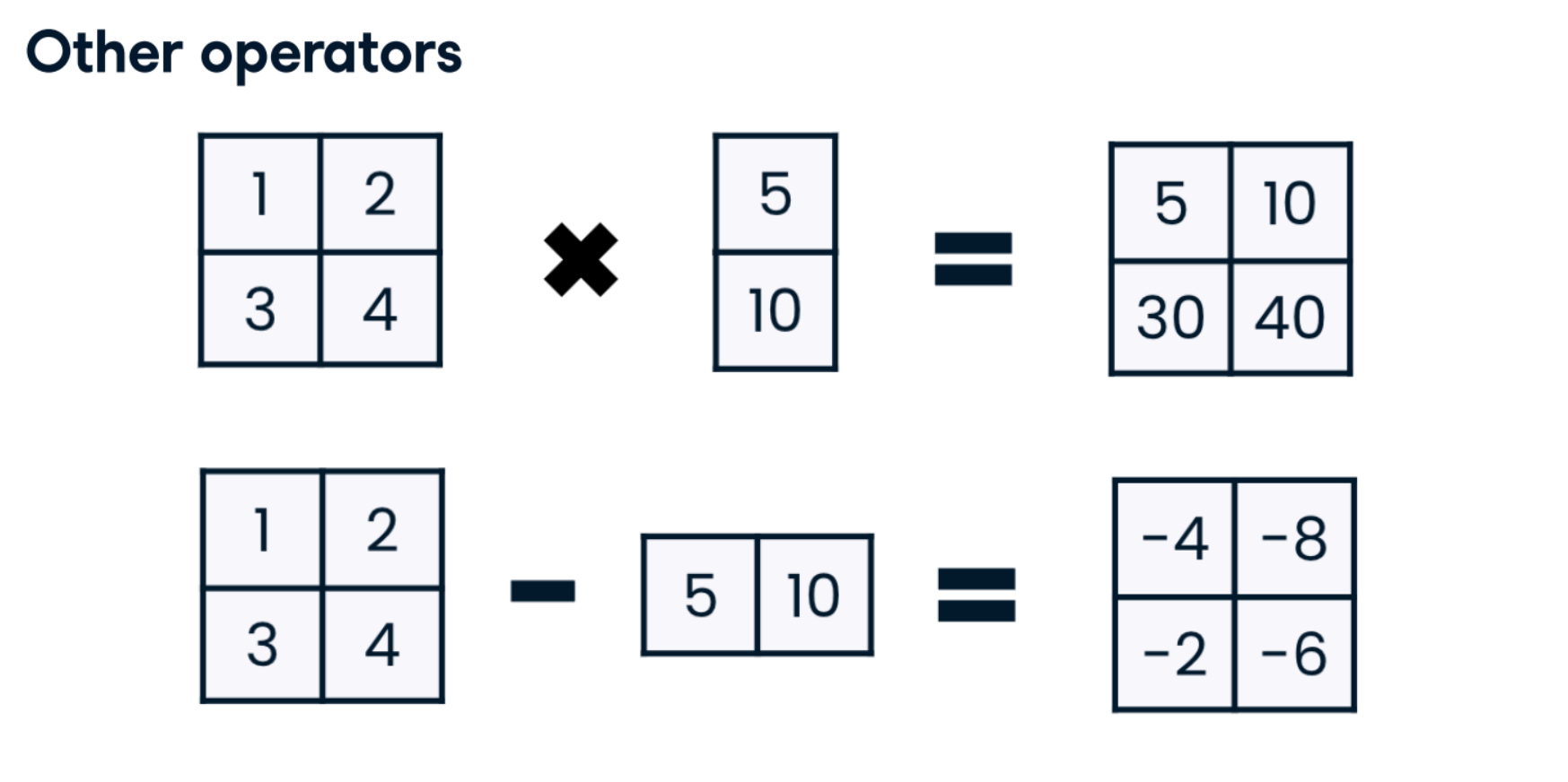
Vectorized operations

- Vectorized operations example
np.arange(1000000).sum()
# 499999500000
For Loops nature are slow
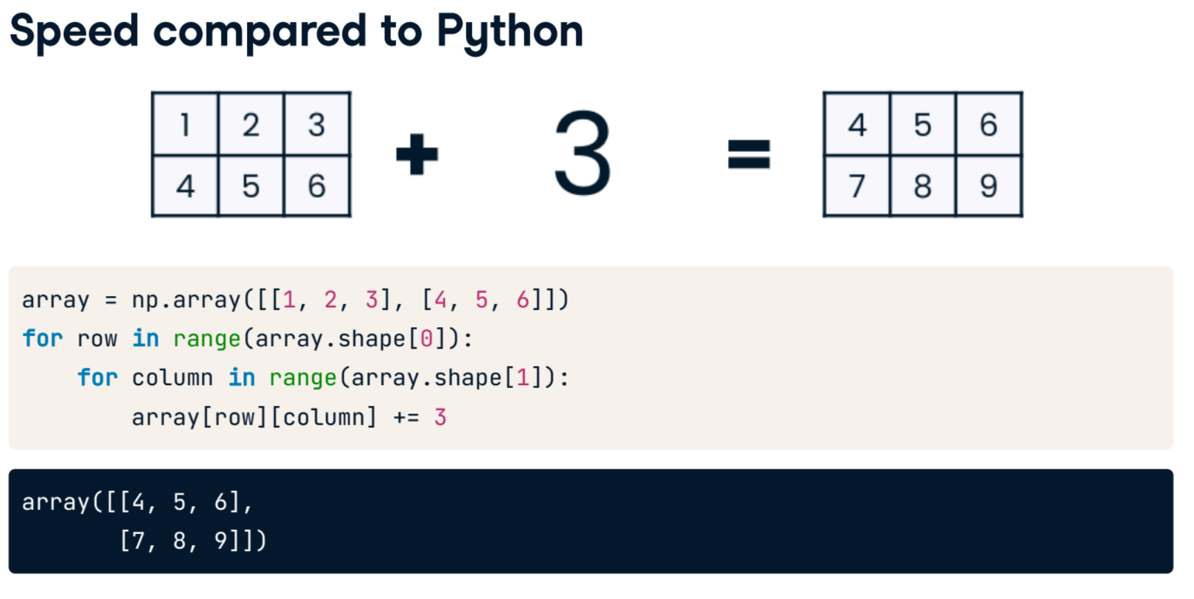
NumPy syntax
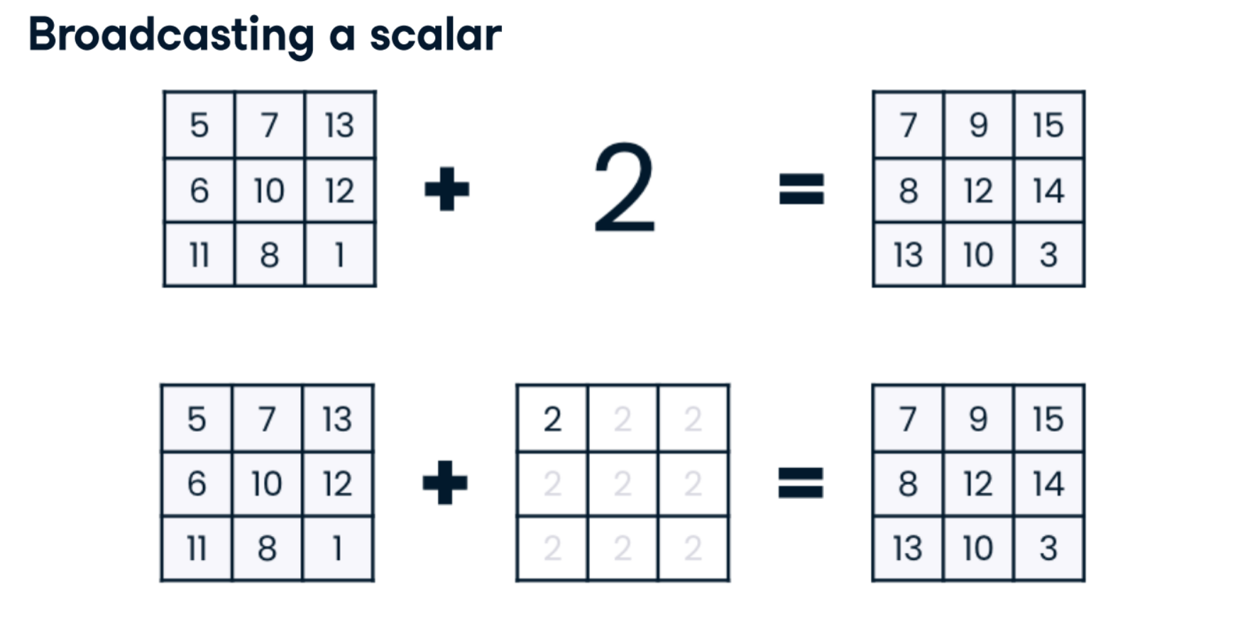
array = np.array([[1, 2, 3],
                [4, 5, 6]])
array + 3
# array([[4, 5, 6],
#        [7, 8, 9]])
Multiplying by a scalar
array = np.array([[1, 2, 3],
                [4, 5, 6]])
array * 3
# array([[ 3, 6, 9],
#       [12, 15, 18]])
Multiplying two arrays together
array_a = np.array([[1, 2, 3], [4, 5, 6]])
array_b = np.array([[0, 1, 0], [1, 0, 1]])
array_a * array_b
# array([[0, 2, 0],[4, 0, 6]])
- Not just for math
Use
npto create boolean mask
array = np.array([[1, 2, 3],
                  [4, 5, 6]])
array > 2

# array([ [False, False, True],
#         [True, True, True]])
- Vectorize Python code!
array = np.array(["NumPy", "is", "awesome"])
len(array) > 2
# True
We can create a vectorized len function
vectorized_len = np.vectorize(len)
vectorized_len(array) > 2
# array([ True, False, True])
Tax calculations
It's possible to use vectorized operations to calculate taxes for the liquor, restaurant, and department store industries! We'll simplify the tax calculation process here and assume that government collects 5% of all sales across these industries as tax revenue.
Your task is to calculate the tax owed by each industry related to each month's sales. numpy is loaded for you as np, and the monthly_sales array is available.
Instructions:
- Create an array called tax_collected which calculates tax collected by industry and month by multiplying each element in monthly_sales by 0.05.
- Create an array that keeps track of total_tax_and_revenue collected by each industry and month by adding each element in tax_collected with its corresponding element in monthly_sales.
tax_collected = monthly_sales * 0.05
print(tax_collected)
total_tax_and_revenue = monthly_sales + tax_collected
print(total_tax_and_revenue)
you've probably noticed that doing mathematical operations with scalars or arrays of the same shape is pretty straightforward. We'll build on this in the next chapter when we explore how NumPy approaches math between two arrays of different shapes!
Projecting sales
You'd like to be able to plan for next year's operations by projecting what sales will be, and you've gathered multipliers specific to each month and industry. These multipliers are saved in an array called monthly_industry_multipliers. For example, the multiplier at monthly_industry_multipliers[0, 0] of 0.98 means that the liquor store industry is projected to have 98% of this January's sales in January of next year.
array([[0.98, 1.02, 1.  ],
       [1.00, 1.01, 0.97],
       [1.06, 1.03, 0.98],
       [1.08, 1.01, 0.98],
       [1.08, 0.98, 0.98],
       [1.1 , 0.99, 0.99],
       [1.12, 1.01, 1.  ],
       [1.1 , 1.02, 1.  ],
       [1.11, 1.01, 1.01],
       [1.08, 0.99, 0.97],
       [1.09, 1.  , 1.02],
       [1.13, 1.03, 1.02]])
numpy is loaded for you as np, and the monthly_sales and monthly_industry_multipliers arrays are available. The monthly_sales columns in order refer to liquor store, restaurant, and department store sales.
Instructions:
- Create an array called projected_monthly_sales which contains projected sales for all three industries based on the multipliers you have gathered.
- Create a graph that plots two lines: current liquor store sales by month and projected liquor store sales by month; months will be represented by an array of the numbers one through twelve.
monthly_industry_multipliers = np.array([[0.98, 1.02, 1.  ],
                                        [1.00, 1.01, 0.97],
                                        [1.06, 1.03, 0.98],
                                        [1.08, 1.01, 0.98],
                                        [1.08, 0.98, 0.98],
                                        [1.1 , 0.99, 0.99],
                                        [1.12, 1.01, 1.  ],
                                        [1.1 , 1.02, 1.  ],
                                        [1.11, 1.01, 1.01],
                                        [1.08, 0.99, 0.97],
                                        [1.09, 1.  , 1.02],
                                        [1.13, 1.03, 1.02]])
projected_monthly_sales = monthly_sales * monthly_industry_multipliers
print(projected_monthly_sales)

# Graph current liquor store sales and projected liquor store sales by month
plt.plot(np.arange(1,13), monthly_sales[:,0], label="Current liquor store sales")
plt.plot(np.arange(1,13), projected_monthly_sales[:,0], label="Projected liquor store sales")
plt.legend()
plt.show()

Well done! It looks like the liquor industry is projected to have a tough January next year. After that, though, projected sales are looking just fine.
Vectorizing .upper()
There are many situations where you might want to use Python methods and functions on array elements in NumPy. You can always write a for loop to do this, but vectorized operations are much faster and more efficient, so consider using np.vectorize()!
You've got an array called names which contains first and last names:
names = np.array([["Izzy", "Monica", "Marvin"],
                  ["Weber", "Patel", "Hernandez"]])
You'd like to use one of the Python methods you learned on DataCamp, .upper(), to make all the letters of every name in the array uppercase. As a reminder, .upper() is a string method, meaning that it must be called on an instance of a string: str.upper().
Your task is to vectorize this Python method. numpy is loaded for you as np, and the names array is available.
Instructions:
- Create a vectorized function called vectorized_upper from the Python .upper() string method.
- Apply vectorized_upper() to the names array and save the resulting array as uppercase_names.
names = np.array([["Izzy", "Monica", "Marvin"],
                  ["Weber", "Patel", "Hernandez"]])
vectorized_upper = np.vectorize(str.upper)

# Apply vectorized_upper to the names array
uppercase_names = vectorized_upper(names)
print(uppercase_names)
Awesome—you can now brag to your friends about how you can vectorize Python functions! You also just harnessed the power of C in your Python code to make it more efficient. Don't forget about np.vectorize() once you've learned to write your own Python functions—you can vectorize those, too!
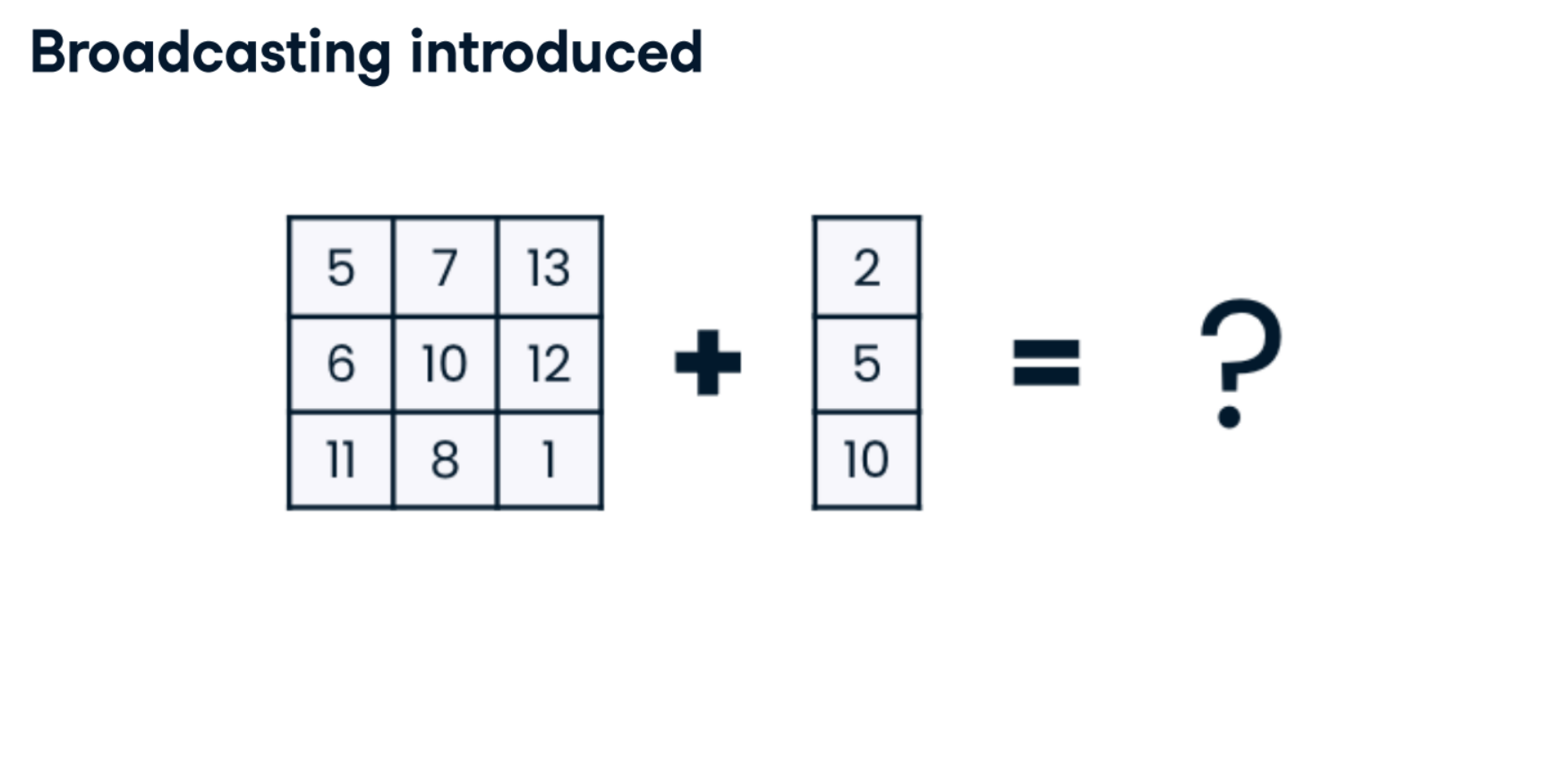
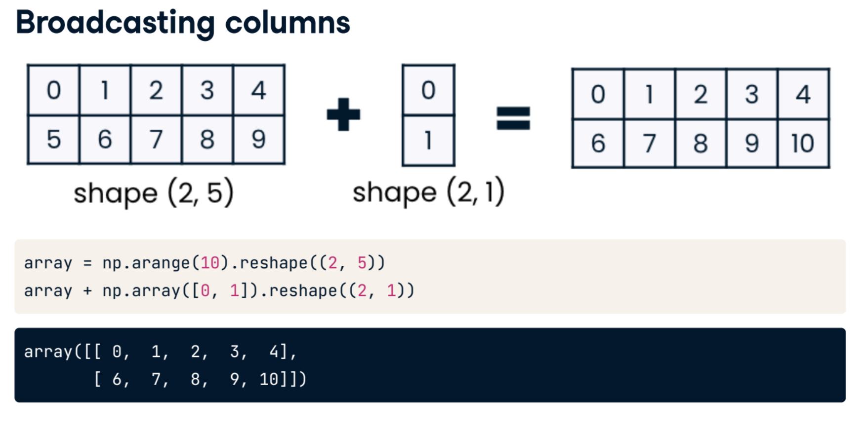
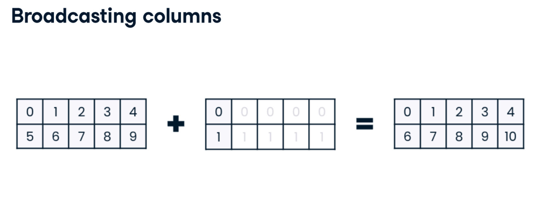
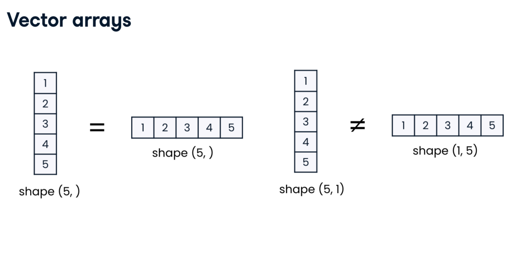
Broadcasting across columns
Recall that when broadcasting across columns, NumPy requires you to be explicit that it should broadcast a vertical array, and horizontal and vertical 1D arrays do not exist in NumPy. Instead, you must first create a 2D array to declare that you have vertical data. Then, NumPy creates a copy of this 2D vertical array for each column and applies the desired operation.
A Python list called monthly_growth_rate with len() of 12 is available. This list represents monthly year-over-year expected growth for the economy; your task is to use broadcasting to multiply this list by each column in the monthly_sales array. The monthly_sales array is loaded, along with numpy as np.
Instructions:
- Convert monthly_growth_rate, currently a Python list, into a one-dimensional NumPy array called monthly_growth_1D.
- Reshape monthly_growth_1D so that it is broadcastable column-wise across monthly_sales; call the new array monthly_growth_2D.
- Using broadcasting, multiply each column in monthly_sales by monthly_growth_2D.
monthly_growth_rate = [1.01, 1.03, 1.03, 1.02, 1.05, 1.03, 1.06, 1.04, 1.03, 1.04, 1.02, 1.01]
# Convert monthly_growth_rate into a NumPy array
monthly_growth_1D = np.array(monthly_growth_rate)

# Reshape monthly_growth_1D
monthly_growth_2D = monthly_growth_1D.reshape((12,1))

# Multiply each column in monthly_sales by monthly_growth_2D
print(monthly_sales * monthly_growth_2D)
Notice how .reshape() was critical here for helping NumPy understand what you wanted it to do. We don't just reshape data for the sake of it!
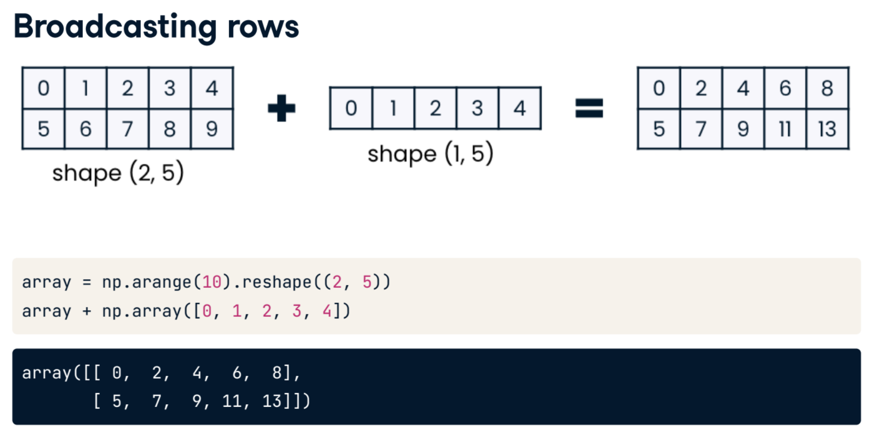
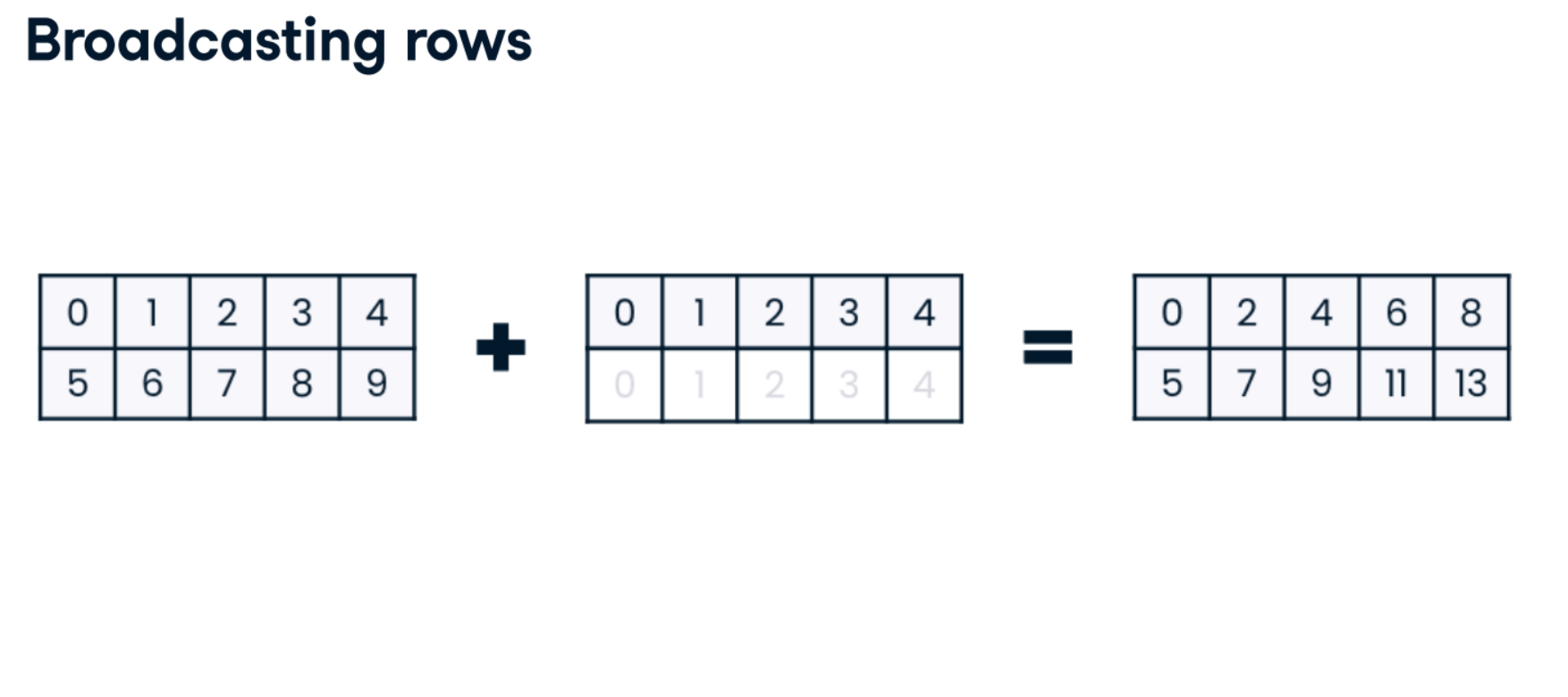
Broadcasting across rows
In the last set of exercises, you used monthly_industry_multipliers, to create sales predictions. Recall that monthly_industry_multipliers looks like this:
array([[0.98, 1.02, 1.  ],
       [1.00, 1.01, 0.97],
       [1.06, 1.03, 0.98],
       [1.08, 1.01, 0.98],
       [1.08, 0.98, 0.98],
       [1.1 , 0.99, 0.99],
       [1.12, 1.01, 1.  ],
       [1.1 , 1.02, 1.  ],
       [1.11, 1.01, 1.01],
       [1.08, 0.99, 0.97],
       [1.09, 1.  , 1.02],
       [1.13, 1.03, 1.02]])
Assume you're not comfortable being so specific with your estimates. Rather, you'd like to use monthly_industry_multipliers to find a single average multiplier for each industry. Then you'll use that multiplier to project next year's sales.
numpy is loaded for you as np, and the monthly_sales and monthly_industry_multipliers arrays are available. The monthly_sales columns in order refer to liquor store, restaurant, and department store sales.
Instructions:
- Find the mean sales projection multiplier for each industry; save in an array called mean_multipliers.
mean_multipliers = monthly_industry_multipliers.mean(axis=0)
print(mean_multipliers)

# Print the shapes of mean_multipliers and monthly_sales
print(mean_multipliers.shape, monthly_sales.shape)

# Multiply each value by the multiplier for that industry
projected_sales = monthly_sales * mean_multipliers
print(projected_sales)
Stellar work! Think about how much code you'd have had to write to perform the same operations on a Python list! Broadcasting is a huge advantage of working with NumPy.
Array Transformations
NumPy meets the art world in this final chapter as we use image data from a Monet masterpiece to explore how you can use to augment image data. You’ll use flipping and transposing functionality to quickly transform our masterpiece. Next, you’ll pull the Monet array apart, make changes, and reconstruct it using array stacking to see the results.
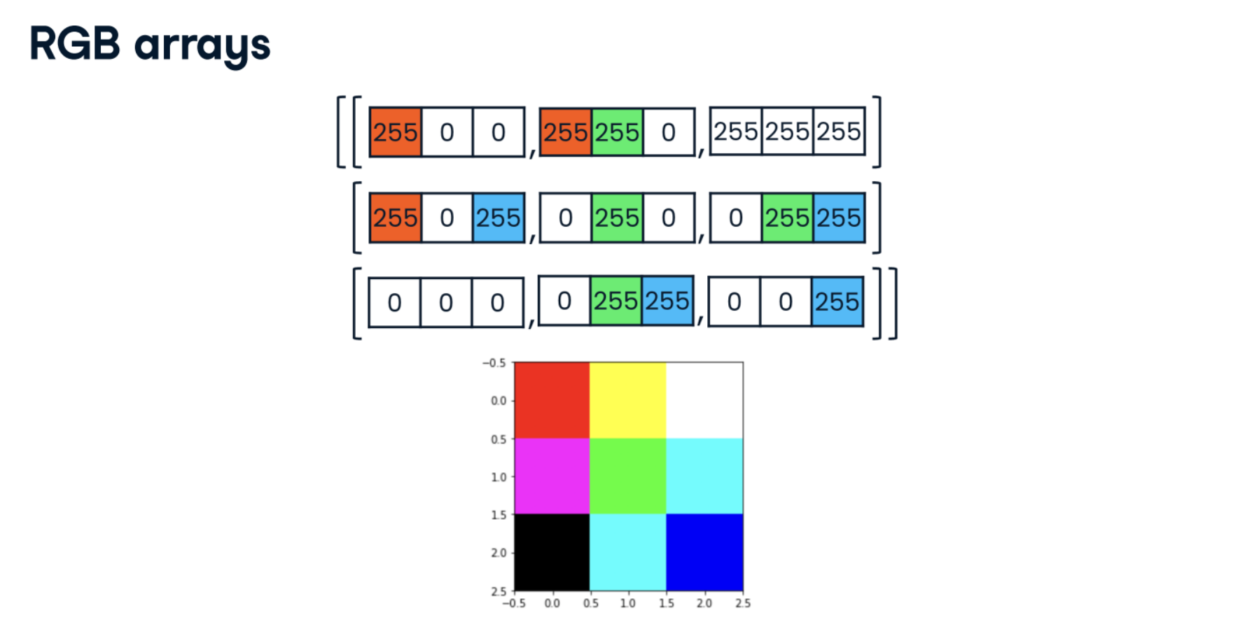
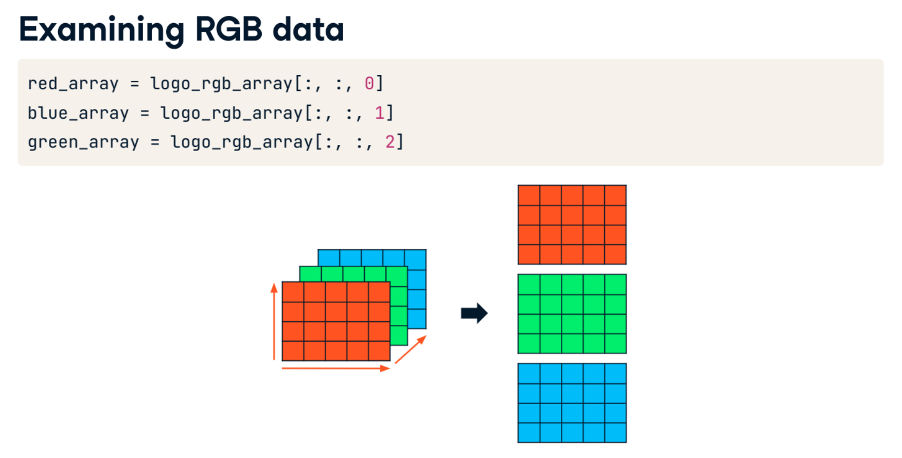
- RGB arrays
rgb = np.array([[[255, 0, 0], [255, 0, 0], [255, 0, 0]],
                [[0, 255, 0], [0, 255, 0], [0, 255, 0]],
                [[0, 0, 255], [0, 0, 255], [0, 0, 255]]])
plt.imshow(rgb)
plt.show()

Saving and loading arrays
- Save arrays in many formats:
- .csv
- .txt
- .pkl
- .npy (best for speed ans size)
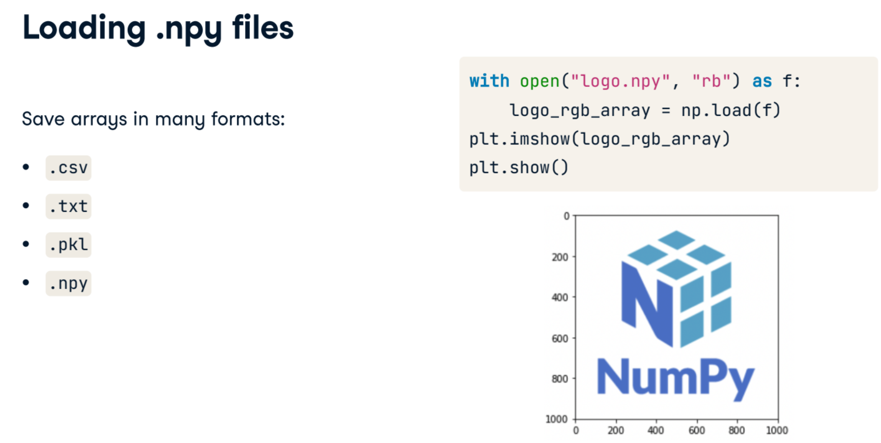
Loading .npy files
with open("logo.npy", "rb") as f:
      logo_rgb_array = np.load(f)
  plt.imshow(logo_rgb_array)
  plt.show()
Saving arrays as .npy files
with open("dark_logo.npy", "wb") as f:
      np.save(f, dark_logo_array)
from PIL import Image
import numpy as np
import cv2
im = cv2.imread('./images/numpy_logo.png')

print(type(im))

print(im.dtype)

print(im.shape)

im_rgb = cv2.cvtColor(im, cv2.COLOR_BGR2RGB)

with open("./datasets/logo.npy", "wb") as f:
    np.save(f, im_rgb)
im2 = cv2.imread('./images/mystery_image.jpg')
im_rgb2 = cv2.cvtColor(im, cv2.COLOR_BGR2RGB)
with open("./datasets/mystery_image.npy", "wb") as f:
    np.save(f, im_rgb2)
with open("./datasets/logo.npy", "rb") as f:
    logo_rgb_array = np.load(f)
plt.imshow(logo_rgb_array)
plt.show()

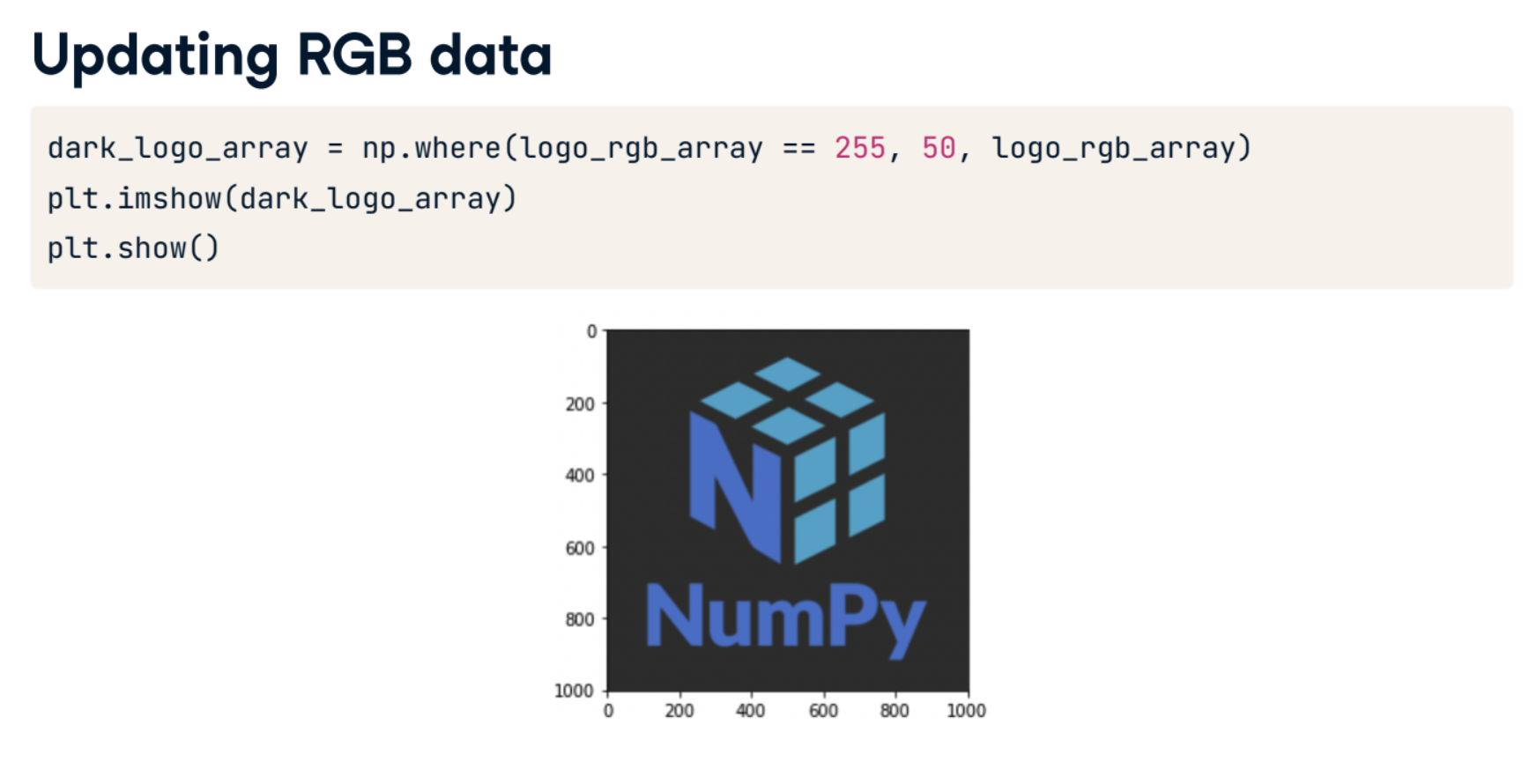
dark_logo_array = np.where(logo_rgb_array == 255, 50, logo_rgb_array)
plt.imshow(dark_logo_array)
plt.show()

with open("./datasets/dark_logo.npy", "wb") as f:
    np.save(f, dark_logo_array)
Loading .npy files
Loading .npy files The exercises for this chapter will use a NumPy array holding an image in RGB format. Which image? You'll have to load the array from the mystery_image.npy file to find out!
numpy is loaded as np, and mystery_image.npy is available.
Instructions:
- Load the mystery_image.npy file using the alias f, saving the contents as an array called
with open("./datasets/mystery_image.npy", "rb") as f:
    rgb_array = np.load(f)

plt.imshow(rgb_array)
plt.show()

- Getting help
You'll need to use the .astype() array method we covered in the first chapter of this course for the next exercise. If you forget exactly how .astype() works, you could check out the course slides or NumPy's documentation on numpy.org. There is, however, an even faster way to jog your memory…
numpy is loaded as np.
# Display the documentation for .astype()
help(np.ndarray.astype)
Armed with that help(), we can move on! Fun fact: if you forget how to use help(), you can always call it with no arguments for a tutorial on how help() itself works.
Update and save
Perhaps you are training a machine learning model to recognize ocean scenes. You'd like the model to understand that oceans are not only associated with bright, summery colors, so you're careful to include images of oceans in bad whether or evening light as well. You may have to manually transform some images in order to balance the data, so your task is to darken the Monet ocean scene rgb_array.
Recall from the video that white is associated with the maximum RGB value of 255, while darker colors are associated with lower values. numpy is loaded as np, and the 3D Monet rgb_array that you loaded in the last exercise is available.
Instructions:
- Reduce every value in rgb_array by 50 percent, saving the resulting array as darker_rgb_array.
- Since RGB values must be integers, convert darker_rgb_array into an array of integers called darker_rgb_int_array so that it can be plotted.
- Save darker_rgb_int_array as an .npy file called darker_monet.npy using the alias f.
darker_rgb_array = rgb_array * 0.5

# Convert darker_rgb_array into an array of integers
darker_rgb_int_array = darker_rgb_array.astype(np.int8)
plt.imshow(darker_rgb_int_array)
plt.show()

# Save darker_rgb_int_array to an .npy file called darker_monet.npy

with open("./datasets/darker_monet.npy", "wb") as f:
    np.save(f, darker_rgb_int_array)

now you've got two different versions of an ocean scene to feed your model! This type of small change can be helpful when the training data you have access to is limited.
plt.imshow(logo_rgb_array)
plt.show()
Flipping an array:
By default,
np.flipflip the array in all axies, sor->g->bwill becomeb->g->r. Also, the rows that formerly appreared at the bottom now will be at the top.
flipped_logo = np.flip(logo_rgb_array)
plt.imshow(flipped_logo)
plt.show()

flipped_rows_logo = np.flip(logo_rgb_array, axis=0)
plt.imshow(flipped_rows_logo)
plt.show()

flipped_colors_logo = np.flip(logo_rgb_array, axis=2)
plt.imshow(flipped_colors_logo)
plt.show()

flipped_except_colors_logo = np.flip(logo_rgb_array, axis=(0, 1))
plt.imshow(flipped_except_colors_logo)
plt.show()

array = np.array([  [1.1, 1.2, 1.3],
                    [2.1, 2.2, 2.3],
                    [3.1, 3.2, 3.3],
                    [4.1, 4.2, 4.3]])
np.flip(array)
array = np.array([  [1.1, 1.2, 1.3],
                    [2.1, 2.2, 2.3],
                    [3.1, 3.2, 3.3],
                    [4.1, 4.2, 4.3]])
np.transpose(array)
transposed_logo = np.transpose(logo_rgb_array, axes=(1, 0, 2))
plt.imshow(transposed_logo)
plt.show()

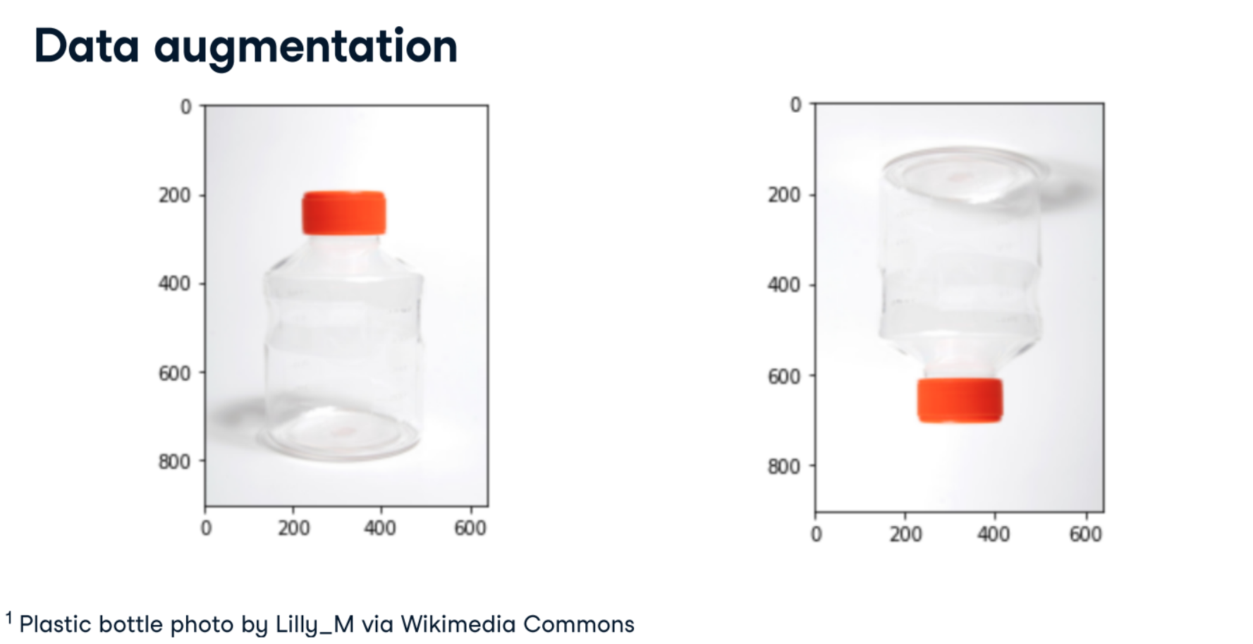
Augmenting Monet
Perhaps you're still working on that machine learning model that identifies ocean scenes in paintings. You'd like to generate a few extra images to augment your existing data. After all, a human can tell that a painting is of an ocean even if the painting is upside-down: why shouldn't your machine learning model?
numpy is loaded as np, and the 3D Monet rgb_array is available.
Instructions:
- Flip rgb_array so that it is the mirror image of the original, with the ocean on the right and grassy knoll on the left.
- Flip rgb_array so that it is upside down but otherwise remains the same.
mirrored_monet = np.flip(rgb_array, axis=1)
plt.imshow(mirrored_monet)
plt.show()

upside_down_monet = np.flip(rgb_array, axis = (0,1))
plt.imshow(upside_down_monet)
plt.show()

The hardest part about flipping arrays is getting the axis right. Checking your work by visualizing your data is always a good idea, even when your data isn't RGB data.
Transposing your masterpiece
ou've learned that transposing an array reverses the order of the array's axes. To transpose the axes in a different order, you can pass the desired axes order as arguments. You'll practice with the 3D Monet rgb_array, loaded for you. numpy has been imported as np.
Instructions:
- Transpose the 3-D rgb_array so that the image appears rotated 90 degrees left and as a mirror image of itself.
transposed_rgb =  np.transpose(rgb_array, axes=(1, 0, 2))
plt.imshow(transposed_rgb)
plt.show()

Great work with tricky 3D data! Even on its side, humans can easily tell that this is a picture of the seaside, despite the unusual placement of the sea, sky, and land. Therefore, this transposed image could be helpful to teach a machine learning model what defines a seaside picture aside from the basic location of the sea, land, and sky.
rgb = np.array([[[255, 0, 0], [255, 255, 0], [255, 255, 255]],
                [[255, 0, 255], [0, 255, 0], [0, 255, 255]],
                [[0, 0, 0], [0, 255, 255], [0, 0, 255]]])

red_array = rgb[:, :, 0]
green_array = rgb[:, :, 1]
blue_array = rgb[:, :, 2]
red_array
red_array2, green_array2, blue_array2 = np.split(rgb, 3, axis=2)
np.array_equal(red_array,red_array2)
red_array.shape
red_array_2D = red_array.reshape((3, 3))
red_array_2D
red_array_2D.shape
- Array division rules
red_array, green_array, blue_array = np.split(rgb, 5, axis=2)
  # ValueError: array split does not result in an equal division
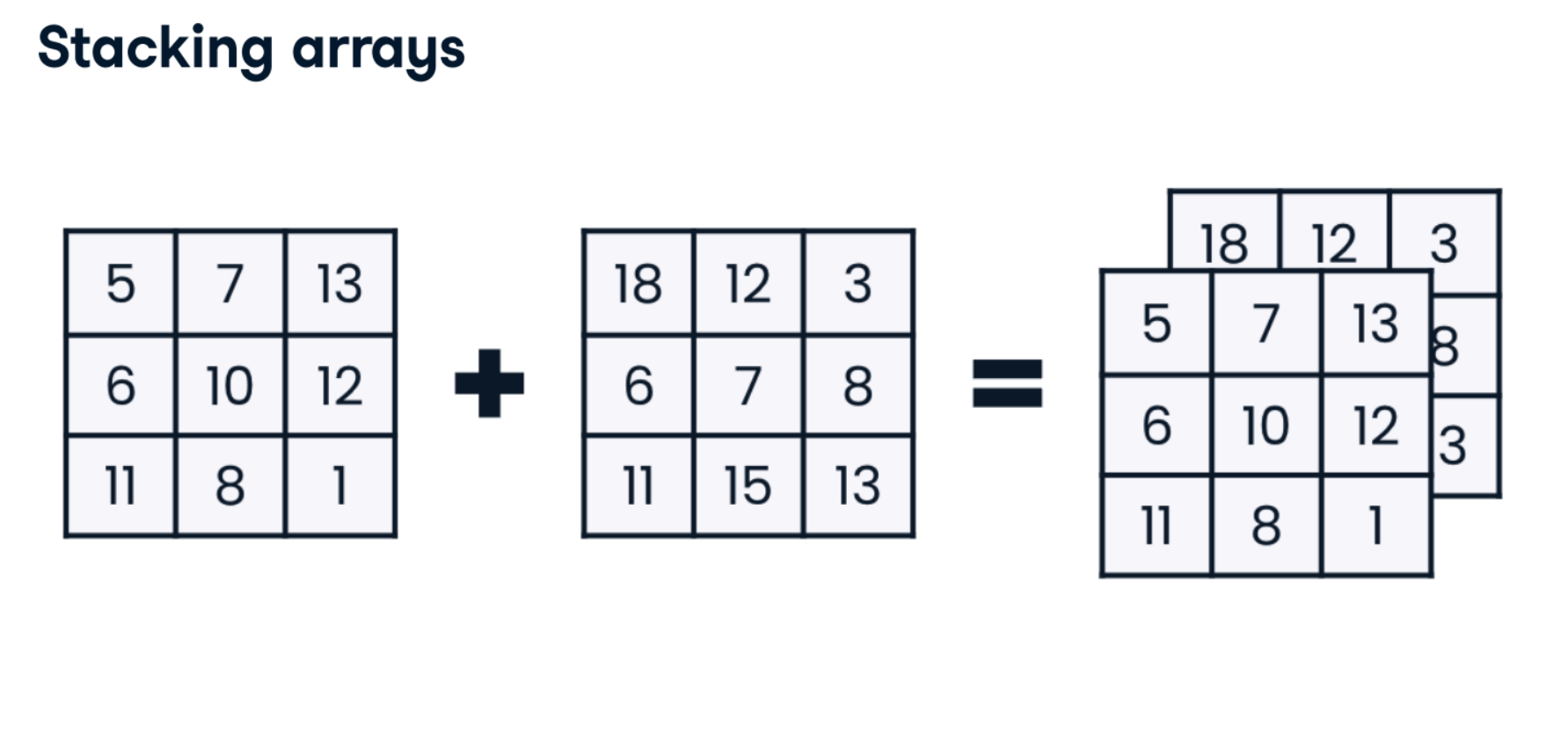
- Stacking arrays
red_array, green_array, blue_array = np.split(logo_rgb_array, 3, axis=2)
plt.imshow(red_array)
plt.show()

red_array = np.zeros((1001, 1001)).astype(np.int32)
green_array = green_array.reshape((1001, 1001))
blue_array = blue_array.reshape((1001, 1001))

stacked_rgb = np.stack([red_array, green_array, blue_array], axis=2)
plt.imshow(stacked_rgb)
plt.show()

2D split and stack
Splitting and stacking skills aren't just useful with 3D RGB arrays: they are excellent for subsetting and organizing data of any type and dimension!
You'll now take a quick trip down memory lane to reorganize the monthly_sales array as a 3D array. Recall that the first dimension of monthly_sales is rows of a single month's sales across three industries, and the second dimension is columns of monthly sales data for a single industry.
Your task is to split this data into quarterly sales data and stack the quarterly sales data so that the new third dimension represents the four 2D arrays of quarterly sales.numpy is loaded as np, and the monthly_sales array is available.
Instructions:
- Split monthly_sales into four arrays representing quarterly data across industries; print q1_sales.
- Stack the four quarterly sales arrays to create a 3D array, quarterly_sales, made up of the four quarterly 2D arrays in order from the first to last quarter.
q1_sales, q2_sales, q3_sales, q4_sales = np.split(monthly_sales, 4)

# Print q1_sales
print(q1_sales)

# Stack the four quarterly sales arrays
quarterly_sales = np.stack([q1_sales, q2_sales, q3_sales, q4_sales])
print(quarterly_sales)
Notice that the above technique is a nice way to reorganize 2D data into 3D data if that's the format your task requires. Now you'll test your skills on 3D RGB arrays...
Splitting RGB data
Perhaps you'd like to better understand Monet's use of the color blue. Your task is to create a version of the Monet rgb_array that emphasizes parts of the painting that use lots of blue by making them even bluer! You'll perform the splitting portion of this task in this exercise and the stacking portion in the next.
numpy is loaded as np, and the Monet rgb_array is available.
Instructions:
- Split the Monet rgb_array into red, green, and blue only pixel data; save the results as as red_array, green_array, and blue_array.
- Create emphasized_blue_array, which replaces blue_array values with 255 if they are higher than the mean value of blue_array; otherwise, the value remains the same.
- Print the .shape of emphasized_blue_array.
- Reshape emphasized_blue_array to remove the trailing third dimension; save as emphasized_blue_array_2D.
red_array, green_array, blue_array = np.split(rgb_array, 3, axis=2)

# Create emphasized_blue_array
emphasized_blue_array = np.where(blue_array > blue_array.mean(), 255, blue_array)

# Print the shape of emphasized_blue_array
print(emphasized_blue_array.shape)

# Remove the trailing dimension from emphasized_blue_array
emphasized_blue_array_2D = emphasized_blue_array.reshape((201, 251))
Stacking RGB data
Now you'll combine red_array, green_array, and emphasized_blue_array_2D to see what Monet's painting looks like with the blues emphasized!
numpy is loaded as np, and the red_array, green_array, blue_array and emphasized_blue_array_2D objects that you created in the last exercise are available.
Instructions:
- Print the shapes of blue_array and emphasized_blue_array_2D.
- Reshape red_array and green_array so that they can be stacked with emphasized_blue_array_2D.
- Stack red_array_2D, green_array_2D, and emphasized_blue_array_2D together (in that order) into a 3D array called emphasized_blue_monet.
print(blue_array.shape, emphasized_blue_array_2D.shape)

# Reshape red_array and green_array
red_array_2D = red_array.reshape((201, 251))
green_array_2D = green_array.reshape((201, 251))

# Stack red_array_2D, green_array_2D, and emphasized_blue_array_2D
emphasized_blue_monet = np.stack([red_array_2D, green_array_2D, emphasized_blue_array_2D], axis = 2)
plt.imshow(emphasized_blue_monet)
plt.show()

Your NumPy skills are really stacking up! Your code did exactly what you asked for: the Monet painting renders very blue in areas that already had high levels of blue, like the sky, but doesn't tint the entire picture blue. Great work!